3. Robust Systems Lab May 28, 2026 10 min

3.21 Monte Carlo for Trading Systems

Monte Carlo has two flavors: bootstrap of trades (IS-distribution) and synthetic paths (model-conditional). Set kill-switches at bootstrap 99th percentile, not IS maximum. Not a substitute for OOS.

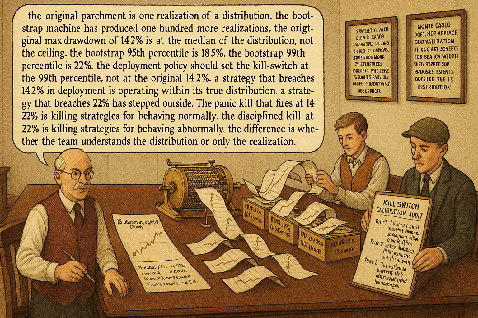
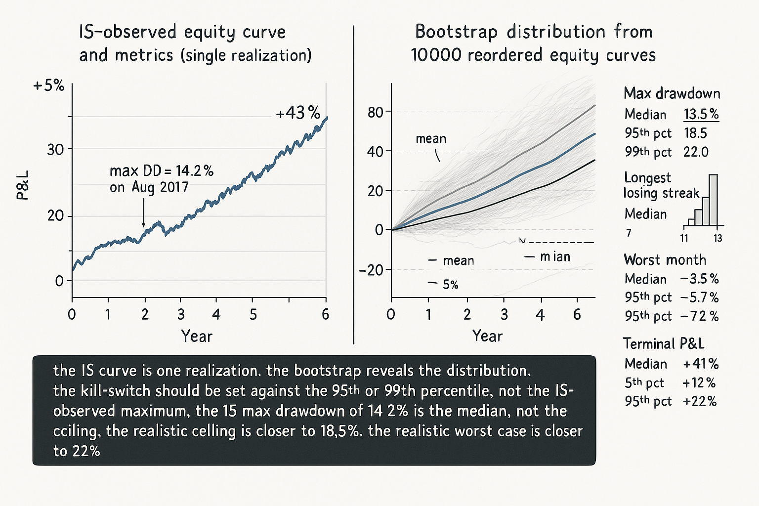
A trading system has 480 trades over 6 years on E-mini SPX futures. The aggregate Sharpe is 1.05, the maximum drawdown is 14.2%, the longest losing streak is 7 trades, the longest losing streak in equity curve is 47 days, and the worst single month was -3.8%. The team prepares a deployment proposal that includes these numbers as the operational risk limits: "expected drawdown ceiling 14.2%, expected worst month -3.8%, expected longest losing streak 7 trades". The risk committee approves with these as the kill-switch thresholds.

The strategy ships. Three months later, the live drawdown reaches 18.5%, exceeding the 14.2% IS-observed limit. The team is forced to either kill the strategy or violate the risk policy. The decision is made in panic. The strategy is killed. Six months after the kill, the same strategy template (re-deployed by another team that did not know the history) reaches Sharpe 1.0 over the next two years, with a max drawdown of 17%. The first team's kill was driven by an IS-observed maximum that was a single realization of a distribution; the actual distribution included drawdowns up to approximately 22% within a one-sigma confidence band. The IS maximum drawdown was an underestimate, not a ceiling.

The article "Trade-Count Thresholds for Backtest Reliability" framed the standard error of the Sharpe; the same logic applies to every other risk metric. The IS-observed maximum drawdown is a noisy realization of the true drawdown distribution. The IS-observed worst month is a noisy realization of the true monthly-return distribution. The IS-observed longest losing streak is a noisy realization of the true losing-streak distribution. Each of these is a single number from a wide distribution. The right operational practice is to estimate the distributions, not the point realizations, and set policy based on the distributional properties. Monte Carlo methods are the standard tool. This article gives the framework for two flavors (bootstrap of historical trades, synthetic-path generation) and the operational uses each enables. The article "Permutation Tests for Indicator Significance" later in this pillar covers a different resampling technique focused on testing whether an indicator has predictive power; the present article covers the resampling techniques focused on understanding the strategy's risk distribution.

Bootstrap Monte Carlo: resampling trades

The simplest Monte Carlo for trading-system risk. The procedure: sample N trades with replacement from the historical N-trade record, in random order, to construct a synthetic equity curve. Repeat 10000 times. Compute the metric of interest (max drawdown, longest losing streak, worst month, terminal P&L) on each synthetic curve. The empirical distribution of the metric across the 10000 synthetic curves is the bootstrap estimate of the metric's sampling distribution.

Bootstrap captures. The bootstrap captures the variation that comes from the order of trades and from the small-sample noise in the per-trade outcomes. A strategy with 480 historical trades has many possible orderings; the IS-observed equity curve is one of them. The bootstrap shows what other orderings would have produced.

Bootstrap blind spots. The bootstrap does not generate trades that did not occur in the IS sample. If the IS sample has no trades during a 2008-style crisis, the bootstrap will not produce 2008-style trades. The bootstrap is conditional on the IS distribution and inherits its limitations. The article "Regime Coverage: Why Your Backtest Needs Different Market States" framed the IS-coverage requirement; the bootstrap does not fix coverage gaps.

The math. Let X_1, X_2, ..., X_N be the per-trade P&L sequence in the IS sample. A bootstrap replication is constructed by drawing N indices uniformly with replacement from {1, ..., N} and forming the sequence X_{i_1}, X_{i_2}, ..., X_{i_N}. The metric of interest f (e.g., max drawdown) is computed on the bootstrapped equity curve.

$$ \widehat{F}_f(x) = \frac{1}{B} \sum_{b=1}^{B} \mathbb{1}\{f(\mathbf{X}^{(b)}) \leq x\} $$

The empirical distribution F_f(x) is the bootstrap estimate of the metric's CDF. From this distribution, percentiles can be computed: the 95th percentile of the max-drawdown distribution is the operationally relevant ceiling, not the IS-observed max-drawdown.

Synthetic-path Monte Carlo: generating returns

A more powerful and more dangerous technique. Instead of resampling historical trades, generate synthetic price paths from a fitted model of the underlying market dynamics. Run the strategy on the synthetic paths. Compute the metric distributions.

Synthetic-path captures. Path-generation models can simulate market events that do not appear in the IS sample (vol regimes outside the IS range, extreme events, regime transitions). With a well-fitted model, the synthetic paths can extend the effective sample size beyond what the historical data alone provides.

Synthetic-path blind spots. The path-generation model is itself a hypothesis about the market's dynamics. If the model is wrong, the synthetic paths are wrong, and the resulting metric distributions are wrong. The article "Slow Wandering: The Most Dangerous Type of Market Change" framed the non-stationarity problem; many path-generation models implicitly assume stationarity, which is the opposite of what real markets exhibit.

Common path-generation models, with their typical biases:

Model 1: GBM (geometric Brownian motion). Simple, well-understood, generates lognormal returns with constant drift and vol. Biases: ignores fat tails, ignores vol clustering, ignores regime breaks. Useful for first-pass scenario analysis; not useful for tail-risk estimation.

Model 2: GARCH-family models. Captures vol clustering. Biases: still assumes the basic return-generating process is stationary, ignores regime breaks, ignores macro-event jumps. Better than GBM for many purposes.

Model 3: jump-diffusion (Merton, Kou). Adds discrete jumps to GBM. Biases: jump sizes and frequencies are calibrated from the IS sample, which underestimates true jump risk if the IS does not include enough jumps.

Model 4: regime-switching models (Hamilton, Markov-switching). Allows regime changes. Biases: number and properties of regimes are calibrated from IS; out-of-sample regimes are not modeled.

Model 5: nonparametric resampling of returns. Sample full days or weeks of returns from history. Captures empirical structure. Biases: same as bootstrap; cannot generate events outside the IS distribution.

The discipline. Use synthetic-path Monte Carlo only when the model assumptions are explicit and the model is calibrated against multiple regimes. Report the model along with the metric distributions; do not present synthetic-path results as if they were data.

Operational uses

Five legitimate applications.

Use 1: confidence intervals on risk metrics. The bootstrap distribution of the max drawdown gives the 95th-percentile drawdown, the 99th-percentile drawdown, and the median. The risk policy uses the 95th or 99th percentile (the realistic ceiling) rather than the IS-observed maximum (a single realization). For the SPX strategy in the opening, the bootstrap 95th-percentile max drawdown might be 18.5%, the 99th-percentile 22%, and the IS-observed 14.2% is the median. The risk policy should be set against the 95th or 99th percentile.

Use 2: sequence-of-returns analysis. The bootstrap reveals how sensitive the equity curve is to the order of trades. A strategy with high terminal P&L but tight bootstrap variation in max drawdown is robust. A strategy with the same terminal P&L but wide bootstrap variation in max drawdown is fragile to bad luck in trade ordering. The fragility is a real operational concern that the IS curve hides.

Use 3: position-sizing calibration. Combined with a Kelly or fractional-Kelly sizing scheme, the bootstrap distribution of equity-curve outcomes informs the right leverage. If the 5th percentile of bootstrap-equity-curve terminal P&L is severely negative under a given leverage, the leverage is too high.

Use 4: kill-switch threshold setting. Use the bootstrap distribution of (max drawdown, time to recover, longest losing streak) to set kill-switch thresholds at the 95th or 99th percentile of the IS-distribution. A breach of the threshold is then strong evidence the strategy is operating outside the IS regime, beyond unlucky variance within it.

Use 5: scenario stress testing. Use synthetic-path Monte Carlo with explicit stress regimes (high-vol, high-correlation, regime-break) to estimate strategy behavior in events not seen in the IS sample. The stress tests are conditional on the model assumptions; the results are not predictions but bounds.

Monte Carlo's limits

Three honest limits.

Limit 1: out-of-sample validation. Monte Carlo is conditional on the IS distribution. It does not provide an independent test of whether the strategy generalizes to OOS regimes. The article "Why OOS Failure Is Often a Stationarity Failure" framed the OOS validation; Monte Carlo informs the IS-distribution diagnostics, not the OOS test.

Limit 2: search-width-bias correction. Monte Carlo on the IS-optimal parameters inherits the IS-optimization bias. The Sharpe distribution from a bootstrap of an over-optimized strategy is centered on the over-optimized IS Sharpe, not on the true Sharpe. The article "Degrees of Freedom in Trading Systems" framed the bias; bootstrap does not remove it.

Limit 3: regime-coverage gaps. If the IS sample has no 2008-style trades, no Monte Carlo can produce them. The technique extends what is in the data, not what is missing.

Anti-patterns

Five mistakes specific to Monte Carlo applications.

Anti-pattern 1: presenting Monte Carlo results as if they were OOS validation. The bootstrap of IS trades is not OOS. It is a refinement of the IS analysis. Reporting it alongside genuine OOS results without distinguishing the two misleads the reader.

Anti-pattern 2: using GBM for tail-risk estimation. GBM has thin tails; real markets have fat tails. The 99th-percentile drawdown from a GBM-based Monte Carlo is severely underestimated. Use jump-diffusion or empirical resampling for tail-risk work.

Anti-pattern 3: bootstrapping with replacement when the trades are serially correlated. The bootstrap assumes i.i.d. observations. Trades that exhibit autocorrelation (consecutive losses cluster, regime-conditional bursts) violate this. Use block-bootstrap (resample contiguous blocks of trades) instead of trade-by-trade bootstrap.

Anti-pattern 4: choosing model assumptions to match the desired result. A team that wants to claim the strategy is robust may select a path-generation model that produces flattering metric distributions. The right discipline is to specify the model and its assumptions before running the simulation, not to choose the model that produces the desired output.

Anti-pattern 5: treating 10000 Monte Carlo replications as "10000x more data". The replications are reordered or re-simulated versions of the same underlying information, with no addition of independent observations. The effective information content is approximately the IS sample, not 10000 times the IS sample. Bootstrap CIs are estimates of the IS-distribution properties, not estimates with 10000-trade-equivalent precision.

Decision matrix

Question	Right MC technique	Wrong MC technique
Confidence interval on max drawdown	Bootstrap of historical trades	GBM-based synthetic paths
Tail-risk estimation (99th pct)	Jump-diffusion or empirical resampling	GBM (thin tails)
Sensitivity to trade ordering	Bootstrap (i.i.d. or block)	Single equity curve
Stress testing rare events	Regime-switching synthetic paths with explicit regimes	Bootstrap (cannot extrapolate)
Position-sizing calibration	Bootstrap with leverage scaling	IS-observed metrics only
Kill-switch threshold setting	Bootstrap 95th/99th percentile	IS-observed maximum
Out-of-sample validation	OOS hold-out, not MC	Bootstrap presented as OOS
Search-width-bias correction	Bias formula from DoF count, not MC	MC of optimized parameters
Strategy comparison (which is better)	Bootstrap-paired comparison	Single-realization comparison

The matrix maps question to right technique. The pattern: bootstrap for IS-distribution diagnostics, synthetic paths only with explicit model and stress-regime context, never as a substitute for OOS validation.

Visualizing the Monte Carlo result

KEY POINTS

Monte Carlo for trading systems comes in two flavors: bootstrap of historical trades (resample with replacement to construct synthetic equity curves) and synthetic-path generation (simulate price paths from a fitted model and run the strategy on them).
The bootstrap captures variation from trade ordering and small-sample noise in per-trade outcomes. It does not capture trades that did not occur in the IS sample. It is conditional on the IS distribution and inherits its coverage limitations.
The synthetic-path approach can extend beyond the IS sample if the path-generation model is well-calibrated. Common models: GBM (thin tails, no clustering), GARCH (captures clustering, ignores regime breaks), jump-diffusion (adds jumps), regime-switching (allows regime changes), nonparametric resampling. Each has documented biases.
Five operational uses: confidence intervals on risk metrics (95th/99th percentile of max drawdown, longest losing streak, worst month), sequence-of-returns analysis (sensitivity of equity curve to trade order), position-sizing calibration (Kelly leverage informed by bootstrap distribution), kill-switch threshold setting (breach indicates regime change, not bad luck), scenario stress testing (synthetic paths with explicit stress regimes).
The IS-observed maximum drawdown is a single realization of the true drawdown distribution. The right operational ceiling is the bootstrap 95th or 99th percentile, not the IS-observed maximum. Setting policy on the IS maximum produces panic kills when the strategy operates within its true distribution.
For a strategy with 480 trades and IS max drawdown 14.2%, the bootstrap distribution might show median 13.5%, 95th percentile 18.5%, 99th percentile 22%. The IS-observed value is the median, not the ceiling.
Monte Carlo cannot replace three things: out-of-sample validation (MC is conditional on IS distribution), search-width-bias correction (MC of an over-optimized strategy inherits the bias), regime-coverage gaps (no MC can produce events outside the IS distribution).
Anti-pattern: presenting MC results as OOS validation. MC is a refinement of IS analysis, not a substitute for hold-out testing.
Anti-pattern: using GBM for tail-risk. GBM has thin tails; real markets have fat tails. Use jump-diffusion or empirical resampling.
Anti-pattern: bootstrapping i.i.d. when trades are serially correlated. Use block-bootstrap (contiguous blocks).
Anti-pattern: choosing model assumptions to match the desired result. Specify the model before running the simulation.
Anti-pattern: treating 10000 replications as 10000x more data. The replications are reorderings of the same underlying information; effective information content equals the IS sample.
The current article gives the resampling techniques for understanding strategy risk. The next article in the publication ("Permutation Tests for Indicator Significance") covers a different resampling technique focused on testing whether an indicator has predictive power against the null hypothesis of no signal.