3.22 Permutation Tests for Indicator Significance
Permutation tests build the null by reordering the indicator while keeping returns fixed. No normality or i.i.d. assumed. Use block permutation for autocorrelated indicators. Pair with effect size.
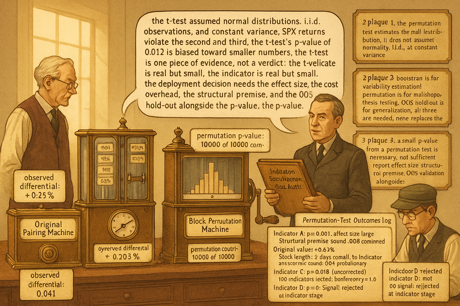
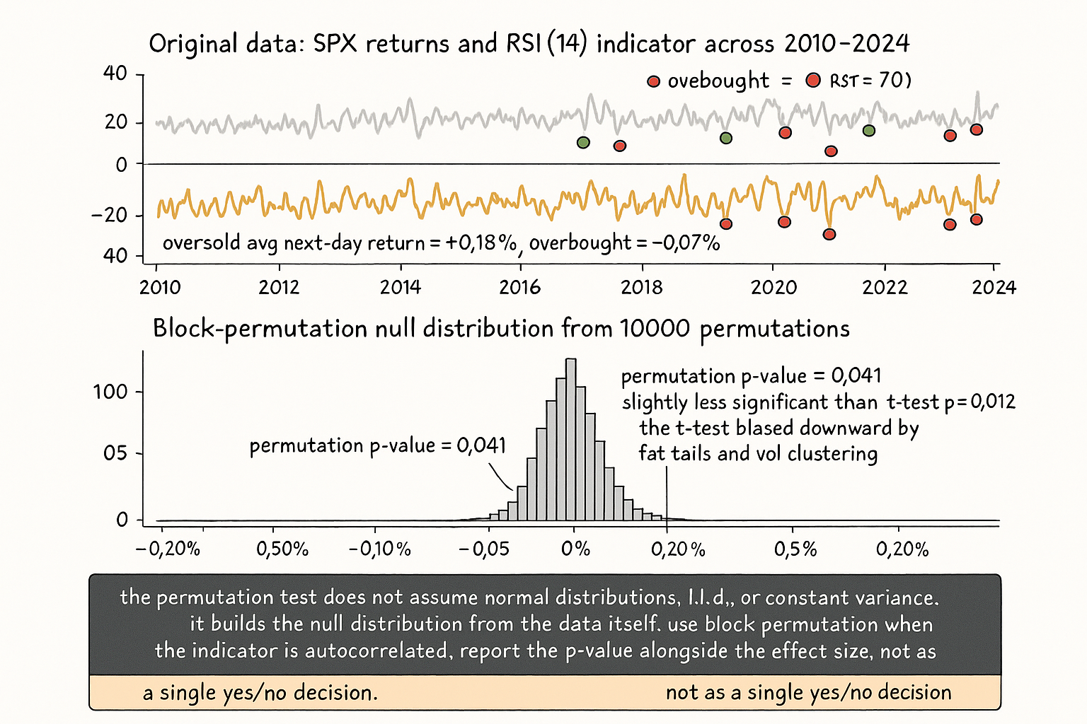
A researcher tests whether a 14-day RSI indicator predicts the next-day return on SPX over 2010-2024. The protocol: compute RSI(14) on each trading day, classify each day as "RSI < 30" (oversold), "RSI in [30, 70]" (neutral), or "RSI > 70" (overbought). Compute the average next-day return in each bucket. The result: oversold days have average next-day return +0.18%, neutral +0.04%, overbought -0.07%. The differential between oversold and overbought is 0.25%. The researcher's question: is the 0.25% differential a real signal, or is it within the range of differentials that would arise by chance even if the indicator had no predictive power?
The standard approach is a t-test, comparing the means of the two buckets. The t-test reports a t-statistic and a p-value. For this dataset (~3500 trading days, ~250 oversold, ~250 overbought, sigma per-day approximately 1.1%), the t-statistic is approximately 2.5 and the p-value is approximately 0.012. Conventional interpretation: significant at the 5% level, marginally significant at the 1% level.
The t-test makes assumptions: i.i.d. observations, normal-or-near-normal return distribution, no serial correlation. SPX returns violate the second and third assumptions. Returns have fat tails (kurtosis approximately 5-7 vs the normal value of 3) and exhibit volatility clustering (next-day return autocorrelation is small but the squared-return autocorrelation is substantial). The t-test's p-value is biased; the true p-value (the actual rate at which the observed differential would arise by chance under the null) is different from the t-test estimate. The article "Why Volatility Is More Non-Stationary Than Trend" framed the autocorrelation structure of squared returns; the same structure invalidates the t-test's i.i.d. assumption.
The permutation test does not make these assumptions. The procedure: under the null hypothesis ("the indicator has no predictive power"), the indicator-value-to-return assignment is arbitrary. Permute the indicator values across days while keeping the return sequence fixed. Compute the same statistic (the differential between oversold and overbought next-day returns) on the permuted dataset. Repeat 10000 times. The empirical distribution of the differential across permutations is the distribution under the null. Compare the original (unpermuted) statistic to this null distribution; the p-value is the fraction of permutation statistics that are as extreme as the observed one.
For the SPX-RSI example, the permutation p-value might be 0.04 (less significant than the t-test's 0.012, by a factor of 3 or so), reflecting the fat-tail-and-clustering corrections. The conclusion shifts: the indicator's predictive power is at the boundary of the conventional significance threshold rather than well below it. The differential of 0.25% is real but smaller than the t-test claims.
The article "Monte Carlo for Trading Systems" covered bootstrap and synthetic-path techniques for understanding strategy risk distributions. Permutation tests are a different resampling technique, designed for testing whether an indicator or signal has predictive power against the null hypothesis of no relationship. This article gives the framework, the implementation details, the legitimate uses, and the failure modes.
The permutation test, formally
The procedure formally. Let X = (x_1, x_2, ..., x_T) be the indicator values and Y = (y_1, y_2, ..., y_T) be the return values, both indexed by time. Let s = f(X, Y) be the test statistic of interest (mean of returns conditional on X above threshold, correlation of X and Y, Sharpe of a strategy long when X is above threshold and flat otherwise, etc.).
The null hypothesis. Under H_0, the indicator has no predictive power: knowing x_t provides no information about y_t (or y_{t+1}, depending on the strategy's lag). Operationally, under H_0, any permutation of X across days is equivalent to the original X.
The permutation procedure. For b = 1 to B: 1. Generate a random permutation pi_b of {1, ..., T}. 2. Construct the permuted indicator sequence X^{(b)} = (x_{pi_b(1)}, x_{pi_b(2)}, ..., x_{pi_b(T)}). 3. Compute s^{(b)} = f(X^{(b)}, Y).
The null distribution. The empirical distribution of {s^{(b)} : b = 1, ..., B} is the distribution of s under H_0.
The p-value. The permutation p-value is the fraction of s^{(b)} values that are as extreme as the observed s.
$$ \hat{p} = \frac{1}{B + 1} \left( 1 + \sum_{b=1}^{B} \mathbb{1}\{s^{(b)} \geq s_{\text{obs}}\} \right) $$
The +1 in the numerator and denominator is the conservative correction that handles the case where no permutation exceeds the observed value. With B = 10000 and zero exceedances, the conservative p-value is 1/10001 = 0.0001.
Permutation test, assumptions it skips. Independence of the y_t sequence (the return autocorrelation is preserved because Y is fixed). Normality of the y_t distribution (the test is non-parametric). Constant variance (the y_t volatility clustering is preserved). The test is robust to all of these.
Permutation test, assumptions it makes. Under H_0, the joint distribution of (x_t, y_t) is exchangeable across t. This holds when there is no time-varying relationship between the indicator and the return. It can fail when the indicator and the return have a shared time-varying component (e.g., both are conditional on the same regime variable that is not being controlled for).
Differences from the bootstrap
Three key distinctions.
Distinction 1: what is resampled. The bootstrap (covered in "Monte Carlo for Trading Systems") resamples the data with replacement to estimate sampling distributions of statistics. The permutation test reorders one of the variables to test a null hypothesis of no relationship.
Distinction 2: what is being estimated. The bootstrap estimates the variability of a statistic under repeated sampling from the same population. The permutation test estimates the distribution of a statistic under a null hypothesis. The two answer different questions.
Distinction 3: what assumptions are required. The bootstrap requires that the data are representative of the population. The permutation test requires that under H_0, the labels (the X values in the example) are exchangeable. The exchangeability assumption is sometimes weaker than the i.i.d.-from-a-population assumption, but it can also fail in ways the bootstrap does not.
The choice. Use the bootstrap to estimate confidence intervals on a parameter (Sharpe, max drawdown, win rate). Use the permutation test to test the null hypothesis that an indicator has no predictive power. The two are complementary; neither replaces the other.
Two implementations of the permutation test
Implementation 1: simple permutation. Permute the indicator series X across days while keeping the return series Y fixed. The implementation in the SPX-RSI example.
Strength: simple to implement, computationally cheap.
Weakness: destroys all temporal structure in X. If X has its own autocorrelation (RSI is a smoothed moving average with strong day-to-day autocorrelation), the simple permutation produces null samples with very different X structure than the original. The null distribution corresponds to "no predictive power on a structureless permutation of X", which differs from "no predictive power on the original-structure X". The two and the test may be biased toward rejecting H_0.
Implementation 2: block permutation. Divide the time series into contiguous blocks of length L (e.g., 5 or 10 days). Permute the blocks rather than individual observations. The implementation preserves within-block autocorrelation while breaking between-block predictability.
Strength: preserves the X autocorrelation structure within each block. The null distribution is closer to "no between-block predictive power".
Weakness: requires choosing the block length L. A block too short loses the autocorrelation structure (similar to simple permutation). A block too long produces too few independent permutations (only T/L blocks to permute).
The discipline. For indicators with substantial autocorrelation (most technical indicators), use block permutation. The block length should be approximately the autocorrelation half-life of the indicator, typically 5-20 days for most technical indicators on daily data.
Applications to indicator and strategy testing
Five legitimate uses.
Use 1: testing whether an indicator predicts returns. The opening example. Statistic: mean differential in next-day returns between oversold and overbought buckets. The p-value is the test result for whether the indicator carries predictive signal.
Use 2: testing whether a strategy's Sharpe is non-zero. Statistic: the Sharpe of the strategy on the original data. Permute the indicator (the trigger sequence) across days. Compute the Sharpe of the permuted strategy. Repeat. The fraction of permuted Sharpes that are as high as the original is the p-value for "the strategy has no edge".
Use 3: testing whether a strategy outperforms a benchmark. Statistic: the differential in Sharpe between the strategy and the benchmark. Permute the indicator. Compare the original differential to the null distribution. The fraction of permuted differentials as extreme as the original is the p-value for "the strategy is no better than the benchmark".
Use 4: testing whether two indicators have predictive power beyond what each contributes individually. Statistic: the joint Sharpe of a strategy using both indicators minus the Sharpe of strategies using each indicator individually. Permute one indicator at a time, then both jointly. The pattern of p-values reveals whether the combined indicator has predictive power not in either component.
Use 5: testing whether a strategy outperforms a "lookahead-shuffled" version of itself. Permute the indicator's relationship to its source data (e.g., shift the indicator by a random number of days). The permuted strategy is identical to the original except for the temporal alignment. If the original Sharpe is much higher than the permutation distribution, the indicator's temporal alignment carries information; if not, the apparent edge is alignment-independent (typically a sign of look-ahead bias or a benchmark-replication artifact).
Failure modes
Four ways the permutation test can mislead.
Failure 1: shared regime structure. Both the indicator and the return are conditional on a regime variable (e.g., volatility regime) that is not being controlled for. The permutation breaks the indicator-return relationship but does not break the regime-driven covariation. The null distribution is mis-specified; the test may falsely reject or falsely fail to reject.
Failure 2: ignoring search-width bias. Testing 100 indicators on the same return series and reporting the most significant one without multiple-comparison correction is a multiple-testing problem. The permutation test on the best-of-100 indicator is biased toward small p-values. Apply Bonferroni or Benjamini-Hochberg corrections.
Failure 3: short time series. With T < 100 observations and an indicator with substantial autocorrelation, the block-permutation test has very few independent blocks (T / L < 10), and the null distribution has low resolution. The p-value is unreliable.
Failure 4: misspecified statistic. The permutation test is conditional on the choice of statistic. Choosing the statistic post-hoc (after seeing the data, picking the comparison that produces the largest effect) inflates the apparent significance. Pre-specify the statistic before the test, and report all chosen statistics across the panel, including the non-significant ones.
Anti-patterns
Five mistakes specific to permutation tests.
Anti-pattern 1: applying simple permutation to indicators with strong autocorrelation. The null distribution is mis-specified; the test rejects too easily. Use block permutation with a block length matched to the indicator's autocorrelation half-life.
Anti-pattern 2: confusing the permutation test with the bootstrap. The bootstrap estimates variability under repeated sampling. The permutation test estimates the null distribution. They answer different questions.
Anti-pattern 3: cherry-picking the test statistic. Running multiple statistics (mean, median, Sharpe, win rate, drawdown) and reporting the one with the smallest p-value inflates the significance. Pre-specify the statistic.
Anti-pattern 4: ignoring multiple-testing corrections when testing many indicators. The probability of finding a "significant" indicator at p < 0.05 from 100 tests under the null is approximately 99%. Apply corrections.
Anti-pattern 5: presenting the permutation p-value as proof the strategy works. The p-value tests whether the indicator has any predictive power; it does not test whether the predictive power is large enough to overcome transaction costs, whether the indicator's structural premise is sound, or whether the strategy survives OOS. The p-value is one piece of evidence; the survival diagnostics are the others.
Decision matrix
| Question | Permutation test | Other tools |
|---|---|---|
| Does an indicator predict returns? | Block permutation, signed test statistic | t-test (assumes i.i.d.), correlation test |
| Is a strategy's Sharpe non-zero? | Permutation of indicator series, Sharpe statistic | Bootstrap-based confidence interval |
| Does a strategy beat a benchmark? | Permutation of differential, paired statistic | Information-ratio significance test |
| Are two indicators jointly predictive? | Permutation of each separately and jointly | Multivariate regression with significance |
| Is a strategy's edge alignment-dependent? | Random-shift permutation of indicator | Comparison to lookahead-shuffled version |
| What is the variability of the Sharpe estimate? | Bootstrap (NOT permutation) | Standard-error formula |
| What is the maximum drawdown distribution? | Bootstrap (NOT permutation) | Synthetic-path Monte Carlo |
| What is the OOS performance estimate? | Hold-out validation (NOT permutation) | Walk-forward analysis |
The matrix maps question to right tool. The pattern: permutation tests are for null-hypothesis testing; bootstraps are for variability estimation; OOS hold-outs are for generalization. None replaces the others.
Visualizing the permutation test
KEY POINTS
- The permutation test estimates the distribution of a test statistic under the null hypothesis that an indicator has no predictive power. Procedure: permute the indicator series across time while keeping the return series fixed, compute the statistic on each permutation, the fraction of permutations as extreme as the observed value is the p-value.
- The permutation test does not assume i.i.d. observations, normal distribution, or constant variance. The return series Y is fixed across permutations, so its autocorrelation, fat tails, and volatility clustering are automatically respected. The test is non-parametric.
- The permutation test assumes exchangeability of the (x_t, y_t) pairs under H_0. The assumption can fail when both the indicator and the return are conditional on an unobserved regime variable; in that case the null distribution is mis-specified.
- Bootstrap and permutation are different: bootstrap resamples to estimate sampling-distribution variability of a statistic, permutation reorders to estimate the null distribution under "no relationship". The two answer different questions and complement each other.
- Two implementations: simple permutation (reorder individual observations, fast, but destroys indicator autocorrelation), block permutation (reorder contiguous blocks of length L, preserves within-block autocorrelation, requires choice of L matching the indicator's autocorrelation half-life).
- Five legitimate uses: testing whether an indicator predicts returns, testing whether a strategy's Sharpe is non-zero, testing whether a strategy beats a benchmark, testing whether two indicators are jointly predictive beyond their individual contributions, testing whether a strategy's edge is alignment-dependent (random-shift permutation).
- Four failure modes: shared regime structure (indicator and return both conditional on an unobserved regime), ignoring search-width bias (testing many indicators inflates the significance of the best one), short time series (T < 100 with autocorrelated indicator has too few independent blocks), misspecified statistic (cherry-picking the statistic after seeing the data).
- Anti-pattern: applying simple permutation to indicators with strong autocorrelation. Use block permutation.
- Anti-pattern: confusing the permutation test with the bootstrap. Different tools, different questions.
- Anti-pattern: cherry-picking the test statistic post-hoc. Pre-specify and report all chosen statistics.
- Anti-pattern: ignoring multiple-testing corrections when testing many indicators. Apply Bonferroni or Benjamini-Hochberg.
- Anti-pattern: treating the p-value as proof the strategy works. The p-value tests for any predictive power; it does not certify that the power is large enough to survive costs, that the structural premise is sound, or that the strategy generalizes OOS.
- The current article completes the resampling-techniques arc that began with the bootstrap-and-synthetic-path coverage in "Monte Carlo for Trading Systems". The combination of permutation tests for indicator significance, bootstrap for risk-distribution estimation, and OOS hold-out for generalization gives the operational toolkit for converting an apparent IS edge into a deployment-ready estimate.
References
- Testing and Tuning Market Trading Systems - Timothy Masters (Amazon)
- Data Mining Algorithms in C++ - Timothy Masters (Amazon)
- Futuretesting Quantitative Strategies
- Rational Stein-GARCH Model: Endogenous Power-Law Tails
- Can LLM-based Financial Investing Strategies Outperform ... - arXiv
- A Filtered-Label Calibrated XGBoost Framework with Walk-Forward
- Using Machine Learning to Forecast Market Direction with Efficient
- A Hybrid AI-Driven Trading System Integrating Technical Analysis
- Quantum vs. Classical Machine Learning: A Benchmark Study for
- An Evolutionary Framework for LLM-Driven Alpha Mining - arXiv