2.75 DSP and Digital Filters for Traders: The Primer Nobody Wrote First

Open any serious book on cycles and you hit a wall by page three. The author talks about transfer functions, frequency response, phase lag, and Nyquist, and assumes you already know what a signal is. You don't, because nobody taught you, and the book moves on without you. The articles in this series on low-pass filters, high-pass filters, band-pass filters, and dominant cycle estimation carry the same assumption. A trader who knows arithmetic and "a sine wave is a wiggly line" deserves a way in. This is that way in.

This article ships no new filter. The filter builds live in their own places: the super-smoother in "The Trader's Guide to Low-Pass Filters", the detrending recursion in "High-Pass Filters for Traders", the cycle isolation in "Band-Pass Filters: The Most Underused Tool in Technical Analysis". This one gives you the vocabulary and the mental model underneath all of them. Read it once and those articles stop being a wall.

Two facts up front, because the rest of the article keeps returning to them and you should resent any source that hides them. First, no causal filter predicts the future; it reshapes the past. Second, smoothing costs lag, and in real-time trading that lag is a tax you pay, never zero, no matter what "zero-lag" marketing claims. Hold those two and you already think more clearly about indicators than most of the people selling them.

What you will be able to do after this

You will be able to say why an indicator lags and whether that lag can be reduced. You will read an amplitude-and-phase response chart without flinching. You will know what low-pass, high-pass, and band-pass mean and which trading job each one does. You will know why a cycle shorter than two bars cannot exist in your data. And you will open any cycles chapter and recognize every term in it. No math beyond arithmetic and the idea that a sine wave goes up and down.

The one-sentence thesis

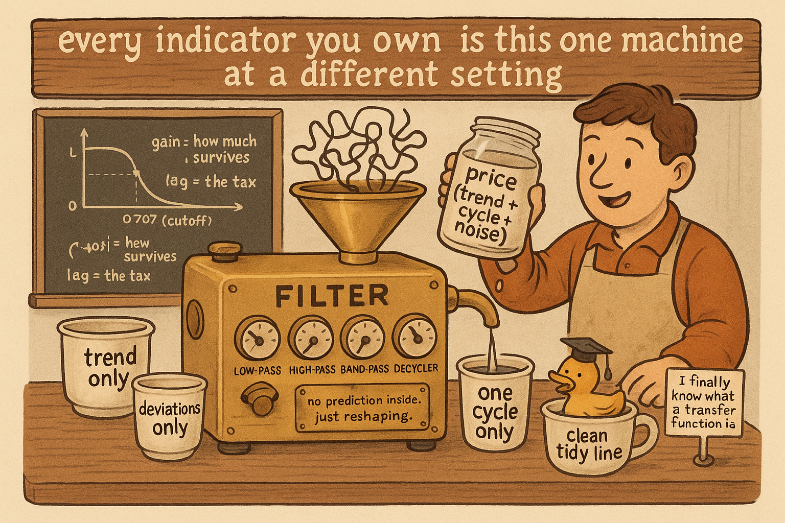
Every indicator you have used is a filter: a machine that takes the price series in and puts a reshaped series out. A moving average is a filter. RSI is a filter wrapped in a nonlinear squashing step. MACD is two filters subtracted. Momentum is a filter. Once you see indicators as filters instead of as named recipes, you stop collecting them and start engineering them, because you can ask the only question that matters: which part of the price did this machine keep, and which part did it throw away?

That reframe is the whole point of this series. A trader who collects indicators owns forty boxes and cannot say what any of them keeps or discards. A trader who thinks in filters owns one idea (reshape the signal) and a handful of dials. The forty boxes turn out to be four machines at different settings.

Price is a signal

A signal is a list of numbers in time order. That is the entire definition. The closing price of the S&P 500, one number per day across years, is a signal. Engineers who design audio gear, radios, and medical scanners work with the same object. They have spent seventy years building tools to reshape those numbers, and almost none of that toolkit was invented for trading, which is why it works on trading; it never saw your backtest and cannot be overfit to it.

Each closing price is a sample. You take one sample per bar, so your sample rate is one sample per bar. On a daily chart that is one sample per day; on a 5-minute chart, one sample every five minutes. The sample rate matters more than beginners expect, and the section on Nyquist below shows why: it sets a hard floor on the fastest wiggle your data can even contain.

Note that closes are not the only choice. You could sample the midpoint, the typical price (high plus low plus close over three), or the volume-weighted price. Each is a different signal built from the same market. For this primer, picture the close, one number per bar, marching left to right.

Signal equals trend plus cycle plus noise

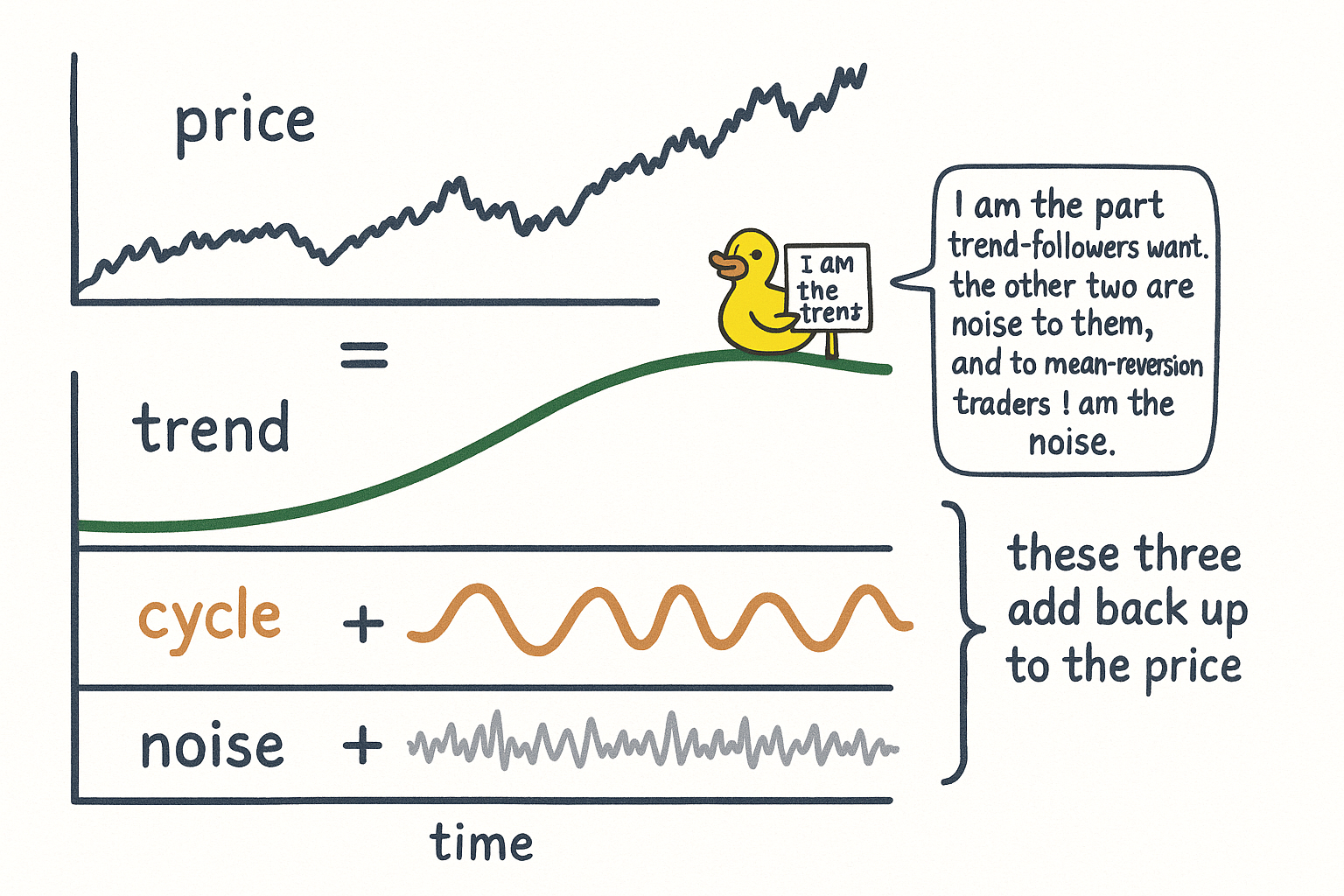
Take any price chart and you can split it into three parts that add back up to the original. A slow drift that bends across the whole window: the trend. A medium wiggle that rises and falls every few dozen bars: the cycle. A fast jitter that changes every bar and looks like static: the noise. Stack those three and you get the price back. Pull them apart and you can see what you are actually trading.

$$ \text{price}[t] \;=\; \text{trend}[t] \;+\; \text{cycle}[t] \;+\; \text{noise}[t] $$

This decomposition is the whole game. A filter is a machine that keeps some of those three parts and kills the rest. A trend follower wants the slow drift and treats the cycle and noise as enemies. A mean-reversion trader on daily equities wants the deviations around the trend and treats the slow drift as the enemy, which is the argument made in detail in "High-Pass Filters for Traders". A cycle trader wants the medium wiggle and treats both the drift and the static as enemies. Same price, three different jobs, three different filters.

The split is not exact and it is not unique. Where the trend ends and the cycle begins is a choice you make by setting a dial (the cutoff), and reasonable people set it differently. That arbitrariness is real and the article on dominant cycle estimation, "Dominant Cycle Estimation Without Astrology", spends its length on how to set the cycle dial from the data instead of by taste.

The wave recipe

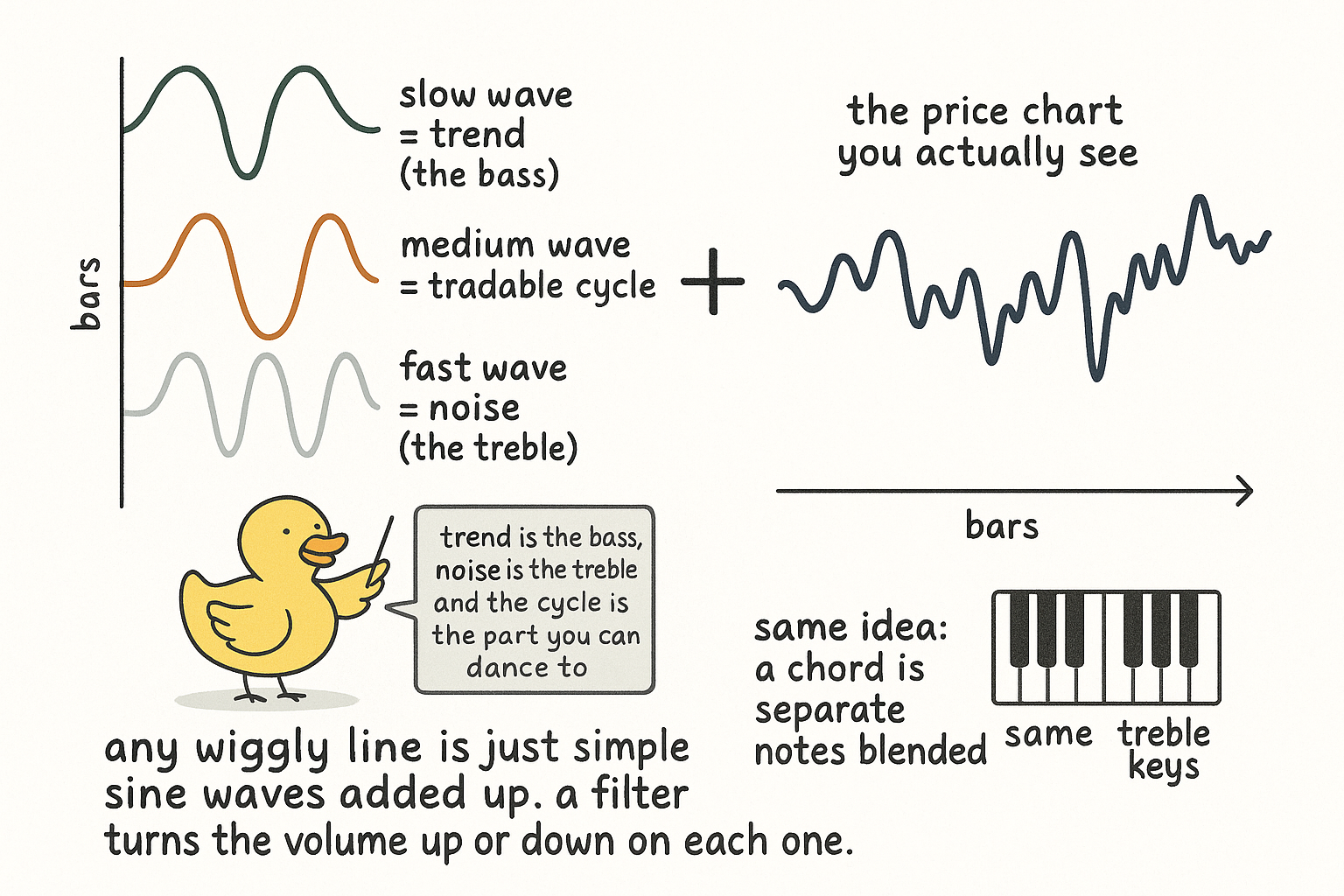
Here is the big idea, and it costs you no math to accept it: any wiggly line, however messy, can be rebuilt by stacking simple sine waves of different speeds and sizes. A slow sine that goes up and down once across the chart, plus a faster one cycling every fifty bars, plus a fast one cycling every three bars, and so on. Add enough of them with the right sizes and you reproduce the original line exactly. This is a mathematical fact, proven two hundred years ago, and you do not need the proof to use it.

Think of the line as a chord played on a piano. The chord sounds like one thing, but it is built from separate notes: a low bass note, some middle notes, a high treble note. Your ear hears the blend; a tuner hears the recipe. The slow sines are the bass (the trend). The fast sines are the treble (the noise). The middle notes are the tradable cycles. The price chart is the chord; the recipe of sines is what filters actually work on.

That recipe has a name: the frequency domain. Looking at the price line itself, value against time, is the time domain, the normal chart you stare at all day. Looking at the recipe instead, how much of each wave speed is present, is the frequency domain. Same information, two views. The time domain answers "what was the price on Tuesday." The frequency domain answers "how much slow drift versus fast noise is in this stretch." A filter is easiest to understand in the frequency domain, because all a filter does is turn the volume up or down on each wave speed. Turn the bass up and the treble down and you have a trend filter. Turn the bass down and the treble up and you have a detrender. That is the entire trick, and the rest of this article makes it precise.

Anatomy of a sine wave

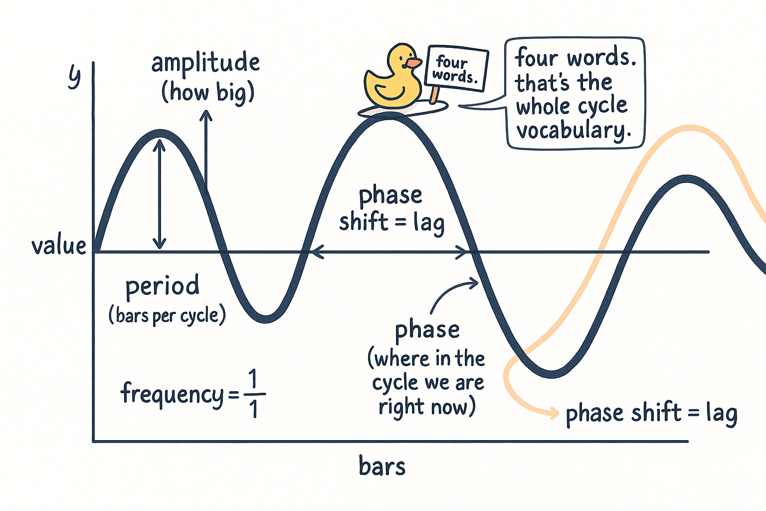
Four words describe a sine wave completely, and they are the entire vocabulary of cycles. Learn these four and the cycle literature opens up.

Amplitude: how big the wave is, the height from the middle to the peak. A high-amplitude cycle swings the price a lot; a low-amplitude one barely moves it.

Period: how many bars one full cycle takes, from one peak to the next peak. A 20-bar period means the wave repeats every 20 bars.

Frequency: how many cycles fit in one bar, which is just one divided by the period. It is the same fact as period, stated upside down.

$$ \text{frequency} \;=\; \frac{1}{\text{period}} $$

A 20-bar period is a frequency of 1/20 = 0.05 cycles per bar. A 4-bar period is 0.25 cycles per bar. Short period means high frequency (fast wiggle); long period means low frequency (slow drift). Traders think in periods because "20-bar cycle" is intuitive; engineers think in frequency because the math is cleaner. You will see both, and the conversion is always this one division. When a chart's x-axis is labeled in frequency from 0 to 0.5, just remember the left side is slow and the right side is fast.

Phase: where in its up-and-down journey the wave sits right now. Two waves with the same period can be out of step, one cresting while the other troughs. Phase measures that offset. Phase matters because lag, the thing you will learn to hate, is a phase shift: a filter that delays the cycle by a quarter of its period has shifted its phase, and that shift is the cost you pay for smoothing.

Sampling, Nyquist, and aliasing

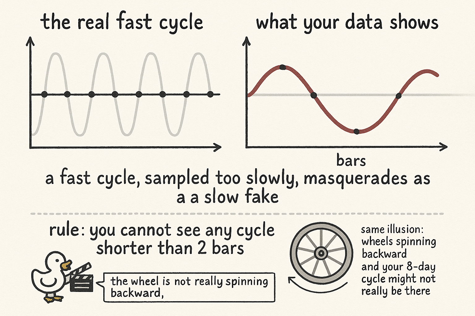
You take one sample per bar. That single fact puts a hard floor on the fastest cycle your data can contain, and the floor is two bars. To see a cycle you need at least one sample on the way up and one on the way down; with one sample per bar, the fastest thing you can resolve goes up on one bar and down on the next, which is a two-bar period. Anything faster than that is invisible to you no matter how good your indicator is. This limit has a name, the Nyquist limit, and for trading it reduces to one rule.

$$ \text{shortest period you can see} \;=\; 2 \text{ bars} $$

This is why every indicator period has a floor and why a "3-bar RSI" is already scraping the bottom of what the data physically holds. It is not a tuning preference; it is a property of sampling once per bar.

Worse than invisibility is disguise. A cycle faster than the two-bar floor does not vanish cleanly when you sample it. It masquerades as a slower cycle that was never there. This is aliasing, and you have seen it: the wagon wheels in old movies that appear to spin backward, or a helicopter rotor that looks frozen on video. The camera samples too slowly, so a fast rotation shows up as a slow or backward one. Your daily close does the same to intraday cycles faster than two days: they fold down and appear as fake multi-day cycles, and you cannot tell them from real ones after the fact.

The practical damage is that a cycle detector can report a clean 8-day cycle that is actually a folded-down intraday cycle, an artifact of sampling, not a feature of the market. The defense is to low-pass filter before you downsample (kill the too-fast content before it can fold), and to distrust any measured cycle near the two-bar floor. The article on why cycles are slippery, "Why Market Cycles Are Evanescent", carries this skepticism further: even a real measured cycle may have already died by the time you act on it.

The lag tax

This is the most important section in the article. Read it twice.

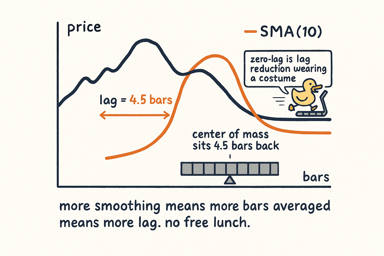
To smooth a series you average over the past. A 10-bar simple moving average at today's bar is the mean of the last ten closes. The output is smoother than the input because the jitter partly cancels when you average. The catch is that the output describes not today but the center of the window you averaged over. Average the last ten bars and the "center of mass" of that window sits 4.5 bars back, so your smooth line reports, on average, where price was four and a half bars ago. That delay is lag, and it is not a bug you can patch. It is the price of averaging.

$$ \text{lag of an SMA of length } N \;=\; \frac{N-1}{2} \text{ bars} $$

For N = 10 that is 4.5 bars. For N = 50 it is 24.5 bars. The arithmetic is brutal and unavoidable: the more you smooth, the more bars you average, the further back the center of mass sits, the more your indicator lags. Smoothness and responsiveness pull in opposite directions, and on a causal filter (one that only sees the past, which is the only kind you can trade) you cannot have both. There is no free lunch.

This is the lie detector for the entire indicator industry. Every "zero-lag" indicator you will ever see is doing lag reduction, not lag elimination. The clever ones extrapolate the recent slope forward to partly cancel the delay, which works when the slope holds and fails exactly when it does not, at turning points, which is when you most wanted the indicator to be right. The article "Why Moving Averages Can Lie at Turning Points" is the full autopsy. For now, hold the rule: in real-time causal filtering, lag is a tax. You can choose how much to pay by trading it against smoothness, but you cannot get the bill to zero.

Note the one honest escape, and why you cannot use it live. A centered filter that averages five bars back and five bars forward has no lag, because its center of mass is today. It also requires knowing five bars of the future, so you can only run it on history, in a chart study, never on the live right edge. Every backtest that quietly uses a centered smoother is cheating, and the cheat is invisible unless you go looking. The non-causal ideal filter (the sinc) is the extreme version of this, and the rigorous DSP cluster covers why you cannot run it in real time.

The four jobs filters do

There are four filter types and each maps to one trading job. Learn the map and you can pick a filter by what you want to keep, instead of by its brand name.

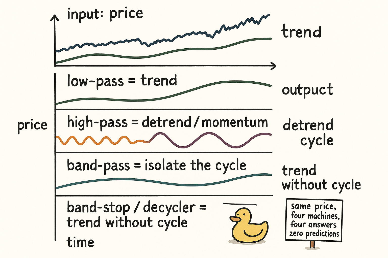
Low-pass: keeps the slow waves, kills the fast ones. The job is trend extraction. Every moving average is a low-pass filter. You use one when the slow drift is the thing you want to trade and the wiggle is in your way. The construction recipe for the good ones lives in "The Trader's Guide to Low-Pass Filters".

High-pass: keeps the fast waves, kills the slow ones. The job is detrending, which gives you momentum and oscillators. You subtract the trend and keep the deviations around it. On daily equities those deviations are where the mean-reversion edge lives, which is the argument in "High-Pass Filters for Traders". The simplest high-pass filter is today's close minus yesterday's close, and the article "No Filter Is Predictive: What Traders Misunderstand About Smoothing" shows why that one-bar difference is the root of every momentum feature.

Band-pass: keeps a chosen middle band of speeds, kills both the slow and the fast. The job is isolating one cycle. You set a center period and a width, and the filter passes wiggles near that period while rejecting both the trend and the noise. This is the core tool for cycle work, built in "Band-Pass Filters: The Most Underused Tool in Technical Analysis".

Band-stop, the decycler version: removes a chosen band and keeps everything else. The job is stripping cycle energy out so the clean trend shows through. Take the price, remove the cycle band, and what remains is a smooth trend line that did not lag the way a moving average would. The construction is in "Decyclers: Extracting Trend by Removing Cycle Energy".

Four jobs, one price. Feed the same chart into all four and you get four different outputs: a smooth trend, a jittery detrended oscillator, a clean isolated cycle, and a decycled trend. None of them predicts anything. Each one keeps a different slice of what was already there.

Frequency response, the filter's fingerprint

Cycle authors put up the same chart constantly and never slow down to teach you how to read it. The chart is the frequency response, and it is the single most useful picture in filter design because it tells you exactly what a filter keeps and what it kills, before you ever run it on data.

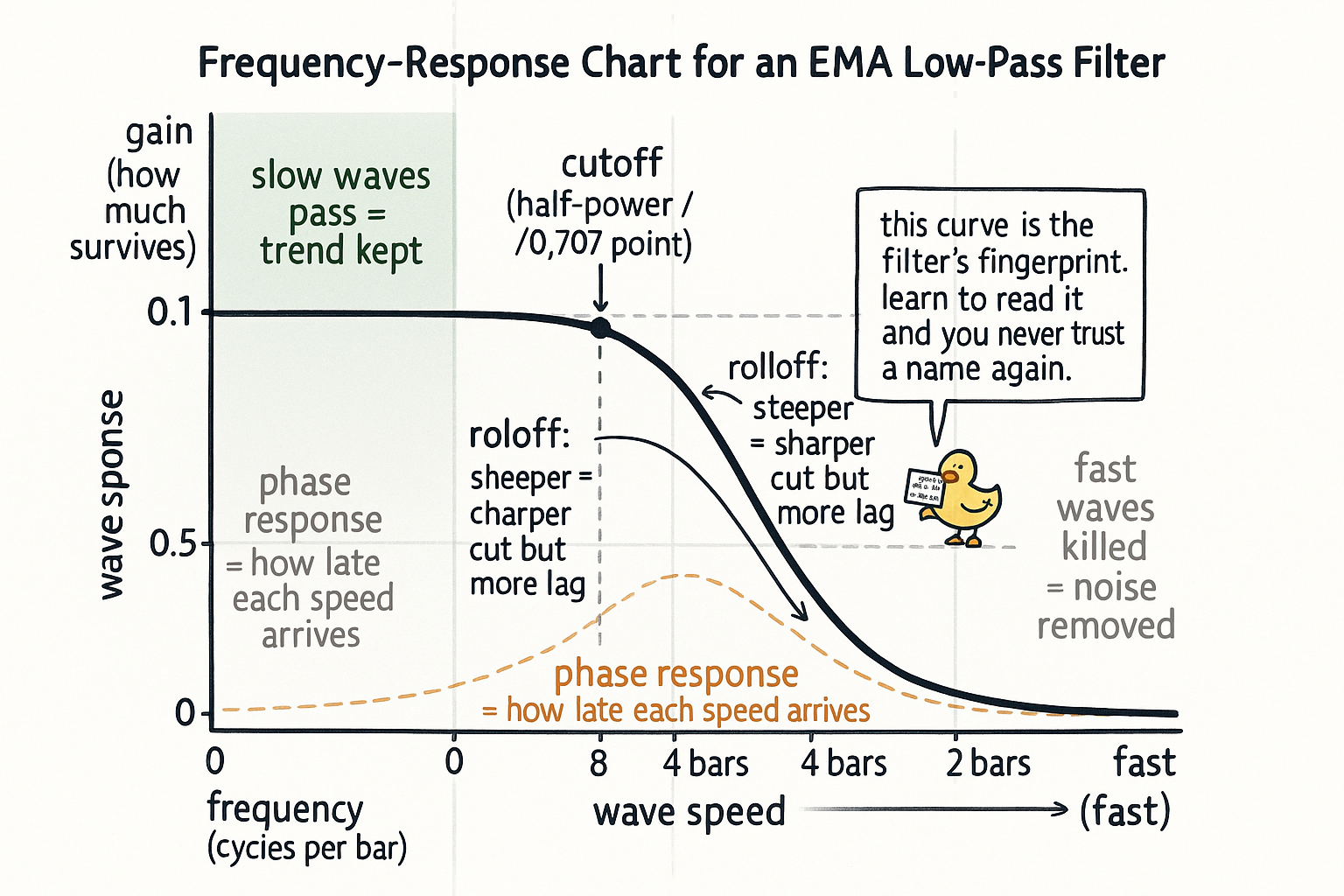
The x-axis is wave speed, labeled either as frequency (0 on the left for slow, up to 0.5 on the right for the fastest two-bar wiggle) or as period (long periods on the left, short on the right). Same axis, two labelings. The y-axis is gain: how much of each speed survives the filter. A gain of 1 means that speed passes untouched. A gain of 0 means that speed is killed dead. A gain of 0.5 means it comes out half as big as it went in. This curve is the amplitude response, and it is the filter's fingerprint.

Read a low-pass filter's fingerprint and the story is plain: gain near 1 on the left (slow waves pass), falling toward 0 on the right (fast waves die). Read a high-pass and it is the mirror: near 0 on the left, near 1 on the right. A band-pass shows a hump in the middle and near 0 on both ends. You can identify any filter's job from the shape of this one curve without knowing a single equation behind it.

Two pieces of standard vocabulary live on this chart. The cutoff, also called the half-power point or the 0.707 point, is the speed where the gain has dropped to about 0.707 of its peak (that number is one over the square root of two, and it marks where the filter has cut the wave's power in half). To the slow side of the cutoff the low-pass mostly passes; to the fast side it mostly blocks; the cutoff is the dividing line you set with the filter's period dial. The rolloff is how steeply the curve falls past the cutoff. A gentle rolloff lets some unwanted content leak through; a steep one cuts harder but, as the lag section warned, costs more lag. You are always trading sharpness against lag, and the frequency response lets you see the trade before you pay for it.

There is a second curve people show alongside the gain: the phase response, how much each speed gets delayed. This is the lag tax drawn as a curve. A filter can pass a cycle at full size (gain 1) while still shifting it late in time (phase delay), which is exactly how a moving average keeps the trend but reports it late. When you read these charts in the cycles literature, gain answers "how much survives" and phase answers "how late does it arrive." The full treatment of reading these on real indicators is "The Frequency Response of Trading Indicators".

FIR versus IIR, in plain words

Two ways exist to build any filter, and the difference shows up in how the filter remembers the past.

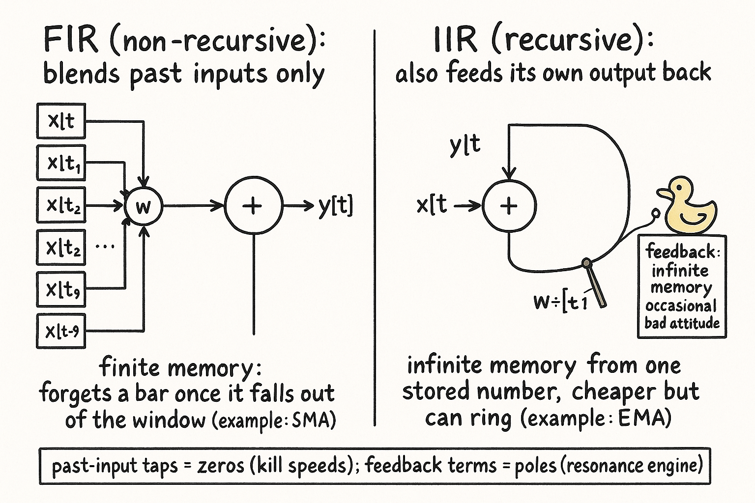
The first kind blends only past inputs. To make today's output you take a weighted mix of the last several closes and nothing else. The simple moving average is the plain example: add the last ten closes, divide by ten, done. This kind is called FIR, finite impulse response, or non-recursive. "Finite" because its memory has a hard end: an SMA of length ten forgets a bar completely once it falls out of the ten-bar window. The weights are out in the open and easy to reason about, which makes FIR filters predictable and stable. The cost is that sharp filtering needs many taps (many past bars in the blend), and many taps means more lag and more computation.

The second kind feeds its own past outputs back in. To make today's output you mix some of today's input with a piece of yesterday's output. The exponential moving average is the example: today's EMA is a fraction of today's close plus the rest of yesterday's EMA. Because yesterday's output already contained a piece of the day before, and so on back forever, this kind has infinite memory from very little storage. It is called IIR, infinite impulse response, or recursive. The payoff is efficiency: an IIR filter gets a sharp response from one or two stored numbers instead of fifty. The risk is that feedback can ring or overshoot, like a pushed swing that keeps swinging, and a badly designed one can go unstable.

A teaser for the math section: the past-input taps of a filter are called its zeros (speeds it kills), and the feedback terms are called its poles (the resonance engine that makes IIR filters efficient and occasionally twitchy). You do not need to compute either one to use this section. Hold the picture: FIR blends the past inputs and forgets cleanly; IIR also recycles its own outputs and remembers forever on the cheap. Almost every Ehlers-style smoother you will meet is IIR, which is why "poles" keeps coming up.

From averages to the z-transform

This is the only section that gets mathy, and it is built one small step at a time. Nothing here is harder than algebra plus one new symbol. The payoff is that you will recognize the transfer function notation that every rigorous filter article uses, even if you never solve one by hand.

Step one, write the filters you already know as equations. The simple moving average of length 3 is just the mean of the last three closes.

$$ y[t] \;=\; \frac{x[t] + x[t-1] + x[t-2]}{3} $$

The exponential moving average mixes a fraction of today's close with the rest of yesterday's output. Call the fraction alpha, a number between 0 and 1.

$$ y[t] \;=\; \alpha \, x[t] \;+\; (1 - \alpha)\, y[t-1] $$

A small alpha (say 0.1) leans hard on the old output and smooths a lot with heavy lag; an alpha near 1 barely smooths at all. That one equation, with one stored number, is the whole EMA. Notice the EMA feeds its own past output back in (the y[t-1] term), which is what made it IIR in the last section.

Step two, the one new symbol. Writing x[t-1] for "yesterday's value" gets clumsy fast, so engineers use a shorthand: the delay operator, written z to the minus one. It means nothing more than "shift back one bar." Multiply a signal by z-to-the-minus-one and you get yesterday's version of it. Multiply by z-to-the-minus-two and you get the value from two bars ago. That is the entire meaning of z at this stage. Do not let the letter scare you; it is a "yesterday" button.

$$ z^{-1} \,x[t] \;=\; x[t-1] \qquad\qquad z^{-2}\,x[t] \;=\; x[t-2] $$

Step three, rewrite the EMA with the delay operator. Replace y[t-1] with z-to-the-minus-one times y, gather the y terms on one side, and you get a compact form.

$$ y \;=\; \alpha\, x \;+\; (1-\alpha)\, z^{-1} y \qquad\Longrightarrow\qquad y \,\big(1 - (1-\alpha) z^{-1}\big) \;=\; \alpha\, x $$

Step four, define the transfer function. Divide output by input and you get a single expression that is the filter's complete DNA. It is called the transfer function, written H of z, and it captures everything the filter does to every wave speed at once.

$$ H(z) \;=\; \frac{y}{x} \;=\; \frac{\alpha}{1 - (1-\alpha)\, z^{-1}} $$

That fraction is the EMA, fully described. The top (numerator) is built from past-input terms. The bottom (denominator) is built from feedback terms. Every linear filter in this entire series can be written this way: a ratio of two short polynomials in the "yesterday" button. When a cycles author writes H(z) and starts factoring it, this is all it is.

Step five, poles and zeros, intuition only. The values of z that make the numerator zero are the zeros: the wave speeds the filter kills dead. The values that make the denominator zero are the poles: the feedback resonances, the engine that lets an IIR filter get a sharp response from almost no storage. A pole sitting close to a cycle speed makes the filter ring at that speed (helpful for a band-pass, dangerous everywhere else). You will leave this section able to look at H(z), point at the numerator and say "those are the zeros," point at the denominator and say "those are the poles," and know which one is the resonance engine. That recognition, not the algebra of solving them, is what unlocks the rigorous articles.

Three worked filters, end to end

Theory earns nothing until you can build it. Here are the three simplest real filters, each as an equation, a one-line description of what it does, and runnable code. The code uses plain Python so you can read it as pseudocode if you do not run it.

The exponential moving average, the 1-pole low-pass. One stored number, one alpha, smooths the series and keeps the trend. This is the filter from the math section above.

def ema(x, alpha):
    y = [x[0]]
    for t in range(1, len(x)):
        y.append(alpha * x[t] + (1 - alpha) * y[t - 1])
    return y

Pass a small alpha for heavy smoothing and heavy lag, a larger alpha for a twitchier, faster line. One pole, gentle rolloff, the cheapest trend filter that exists. Frequency response: gain near 1 for slow waves, sliding down toward 0 for fast ones, a textbook low-pass that fades rather than cuts. The construction details and why traders should prefer it to the SMA in some cases live in "EMA vs SMA: Why Simplicity Still Matters".

Simple momentum, today minus N bars ago, which is secretly a high-pass filter. People think of momentum as a strength gauge; structurally it subtracts the slow level and keeps the change, which is exactly what a detrender does.

def momentum(x, n):
    return [None] * n + [x[t] - x[t - n] for t in range(n, len(x))]

The output is large when price has moved a lot over the last N bars and near zero when it has not. Because it subtracts a delayed copy of the price, the slow drift cancels and the fast change survives: a high-pass filter wearing a momentum label. Frequency response: gain near 0 for slow waves (the trend gets killed) rising for faster ones, the mirror image of the EMA. This is the seed that grows into the full detrending toolkit in "High-Pass Filters for Traders".

A 2-pole smoother, the super-smoother flavor, to show why more poles cut sharper but cost more lag. Two stored numbers, a steeper rolloff than the EMA, much cleaner rejection of fast noise.

import math

def two_pole_smoother(x, period):
    a = math.exp(-1.414 * math.pi / period)
    b = 2 * a * math.cos(1.414 * math.pi / period)
    c2, c3 = b, -a * a
    c1 = 1 - c2 - c3
    y = list(x[:2])
    for t in range(2, len(x)):
        y.append(c1 * (x[t] + x[t - 1]) / 2 + c2 * y[t - 1] + c3 * y[t - 2])
    return y

The two feedback terms (the y[t-1] and y[t-2]) are the two poles. Frequency response: the same low-pass shape as the EMA but with a steeper rolloff past the cutoff, so it holds the trend at full gain longer and then drops fast noise harder. Compared to the 1-pole EMA, this filter passes the trend almost untouched while killing fast noise far harder, at the cost of a bit more lag, exactly the sharpness-versus-lag trade the frequency-response section promised. This is the workhorse low-pass behind the more rigorous smoothers, built out fully in "The Trader's Guide to Low-Pass Filters", and the same two-pole structure reappears in the rigorous DSP cluster on Butterworth and higher-order designs.

Run all three on the same price series and watch the lag tax appear on its own: the heavier the smoothing, the later the line turns. No new theory needed to see it. Reuse the frequency-response idea from earlier and you can predict the shape of each output before you plot it.

Bridge to the rest of the series

You now hold the whole vocabulary. Every term in the cycles literature maps to something you learned above. Here is the payoff map, so the downstream syllabus snaps into place.

Read down that column and you have the reading order. Every one of those articles assumes the vocabulary you now own.

Honest caveats

Five closing truths, because a primer that left you optimistic would have failed you.

No filter predicts. A filter reshapes the history it has seen; it has no term for the future, as "No Filter Is Predictive: What Traders Misunderstand About Smoothing" proves with the algebra. When a smoothed line turns up, it is reporting that the past already turned up, late. Trade the output as a feature, never as a forecast.

Lag is a tax, never zero. On any causal filter you can trade smoothness against responsiveness, but you cannot get the lag to zero. Every "zero-lag" claim is lag reduction that works until the slope it extrapolates breaks, which tends to be the turning point you cared about.

There is no perfect brick-wall filter you can run live. The ideal filter that passes everything below a cutoff and kills everything above, with no transition and no lag, needs future data to build (its shape, the sinc, extends infinitely in both directions). You can run it on history and feel clever; you cannot run it at the live right edge. The rigorous DSP cluster covers why.

Cycles are slippery. A cycle you measure today may already be gone, because market cycles fade in and out rather than persisting like a clock, the argument in "Why Market Cycles Are Evanescent". Measuring a 20-bar cycle does not promise it survives to the next swing.

A filter with a beautiful response can still be a terrible trading feature. Clean frequency response and good predictive value are different questions. A filter can pass exactly the band you wanted and still feed your model noise, because that band carried no edge on your instrument. Whether a feature predicts is an empirical question you answer with the indicator-quality tests in the pillar on building features that actually work, not with the shape of a response curve.

KEY POINTS

• Every indicator is a filter: a machine that takes price in and puts a reshaped series out. Stop collecting indicators, start asking which part of the price each one keeps and kills.
• A signal is numbers in time order. Closes are samples at one sample per bar. The sample rate sets a hard floor on the fastest cycle you can see.
• Any price line splits into trend plus cycle plus noise, and those three add back up. A filter keeps some parts and kills the rest. The split is a choice you set with a dial.
• Any wiggly line rebuilds from stacked sine waves. The recipe of waves is the frequency domain; the price line is the time domain. A filter turns the volume up or down on each wave speed.
• Four words describe any cycle: amplitude (size), period (bars per cycle), frequency (1 over period), phase (where in the cycle it sits now). Lag is a phase shift.
• The shortest cycle your data can hold is 2 bars (Nyquist). Anything faster either vanishes or, worse, masquerades as a slow fake cycle (aliasing, the wagon-wheel effect).
• Lag is the tax on smoothing. An SMA of length N lags by (N-1)/2 bars because its center of mass sits that far back. On a causal filter the lag is never zero; every "zero-lag" claim is lag reduction.
• Four filter jobs: low-pass keeps the trend, high-pass keeps the deviations (momentum, mean reversion), band-pass isolates one cycle, band-stop (decycler) strips the cycle to leave a clean trend.
• The frequency response is the filter's fingerprint: x-axis is wave speed, y-axis is gain (how much survives). The 0.707 point is the cutoff; the rolloff slope trades sharpness against lag.
• FIR (non-recursive, like the SMA) blends past inputs and forgets cleanly. IIR (recursive, like the EMA) recycles its own outputs for infinite memory from almost no storage, cheaper but can ring.
• The transfer function H(z) is a filter's complete DNA: a ratio of two short polynomials in the delay operator z (the "yesterday" button). Numerator terms are zeros (speeds killed); denominator terms are poles (the resonance engine).
• No filter predicts; it reshapes history. Cycles fade. A clean response does not guarantee a profitable feature. Prove predictive value empirically, not from the shape of a curve.

References

• Statistically Sound Indicators for Financial Market Prediction - Timothy Masters (Amazon)
• Cycle Analytics for Traders - John Ehlers (Amazon)
• A Novel Distance-Based Moving Average Model for Improvement in the Predictive Accuracy of Financial Time Series
• Key Technical Indicators for Stock Market Prediction
• Mitigating False Signals in Crypto-Asset Trading Using a Binary Hybrid Financial Signal Processing and Machine Learning Framework
• Hierarchical Endogenous Market-State Representation for Financial Portfolio Management
• Intraday Patterns in Natural Gas Futures: Extracting Signals from High-Frequency Trading Data
• Signal Processing System - an overview | ScienceDirect Topics
• What Is Quality? (Summary)
• FINANCIAL TIME-SERIES PREDICTION USING DEEP LEARNING