2.83 Ehlers Was Building State-Space Models in TradeStation
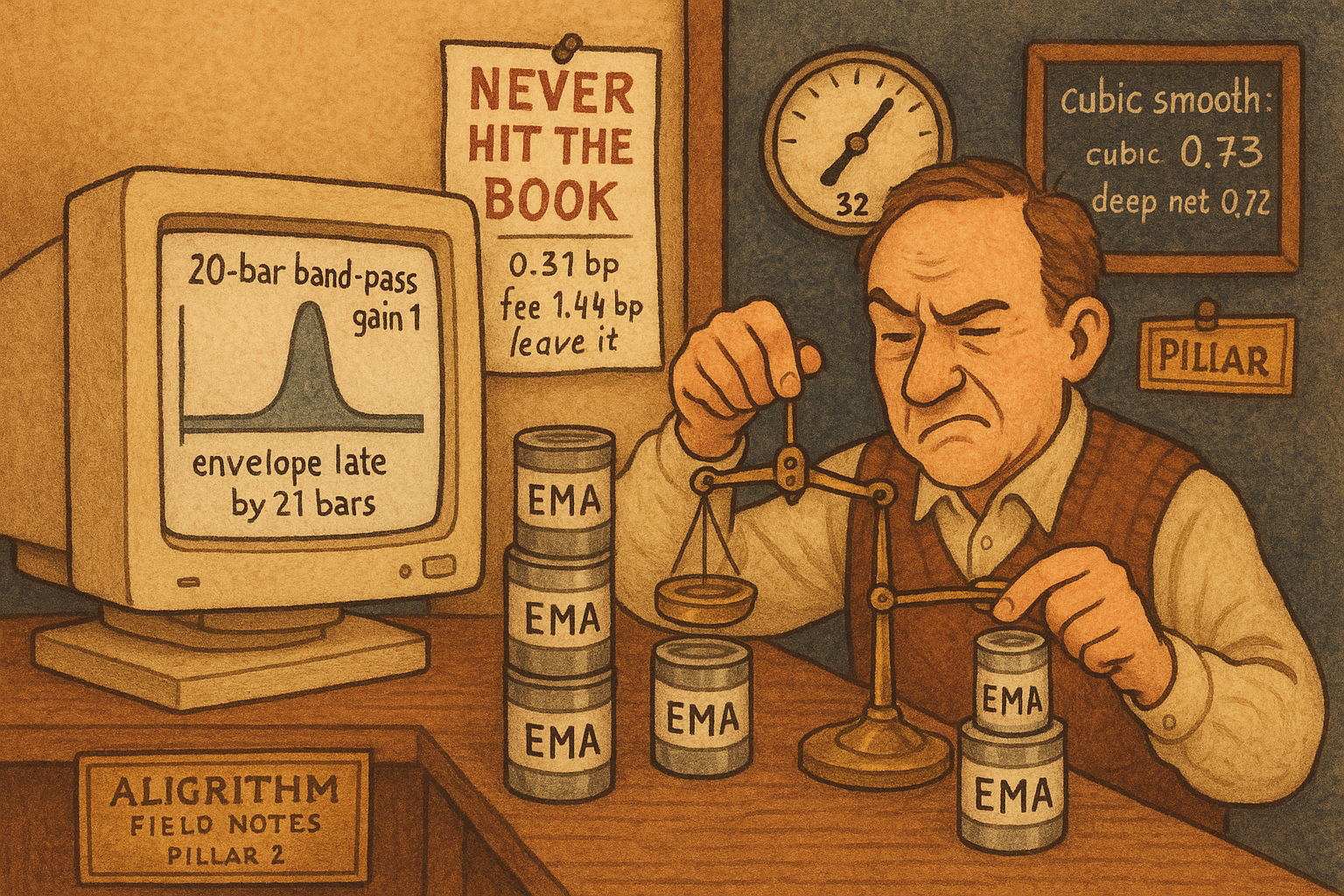
Bitcoin state-space models are filters: a 20-bar band-pass has gain 1 and a 21-bar envelope delay, while a two-real-pole fit to it peaks at 32 bars.
Sepehri, Mehradfar, Soltanolkotabi, and Avestimehr build CryptoMamba on daily Bitcoin, the Yahoo Finance BTC-USD series from 17 September 2018 to 17 September 2024. The memory update they print is a state-space model: each bar, a state vector is multiplied by a matrix and a new input is added. That update is a linear filter. The second-order band-pass in the old article "Band-Pass Filters: The Most Underused Tool in Technical Analysis" is the same update, and a pure 20-bar sine comes out of it at gain 1, meaning the sine is unchanged in size. Constrain the state matrix to two real decays, fit them to that band-pass, and the gain peaks at 32 bars.
A real pole discretizes into an exponential average
A state-space model keeps a memory vector. Call the memory x, the input u, and the output y. Their background equation, written for a scalar input, is the continuous form from control theory.
$$ \dot{x}(t) = A x(t) + B u(t), \qquad y(t) = C x(t) + D u(t) $$
A sets how the memory decays, B sets how the new input enters the memory, C reads the memory out, and D is a direct passthrough they drop once the clock is discrete. On daily bars the input is held constant for one bar. That hold is a zero-order hold. They name the hold and omit the formula for the discrete input weight. The map is below. The bar length is Δ, equal to 1 when the clock is one bar.
$$ x_k = \bar{A}\, x_{k-1} + \bar{B}\, u_k, \qquad \bar{A} = \exp(A \Delta), \qquad \bar{B} = A^{-1}\bigl(\exp(A \Delta) - I\bigr) B $$
The output is C times the new state. Work a scalar pole, the same one the old article "State-Space Models for Price: CryptoMamba vs Transformers (Skeptical)" used. Set A to -0.5, B to 1, and Δ to 1. Then A-bar is exp(-0.5), which is 0.606531. The input weight is (exp(-0.5) - 1) / (-0.5). The numerator is -0.393469, the denominator is -0.5, and B-bar is 0.786938. The old article rounded those to 0.607 and 0.786.
With C left at 1, the zero-frequency gain, the response to a constant, is B-bar / (1 - A-bar) = 0.786938 / 0.393469 = 2 exactly, because (1 - exp(AΔ)) / (-A) divided by (1 - exp(AΔ)) is 1/(-A), and -A is 0.5. Set C to 0.5 and a constant input passes at gain 1.
The trader's form of that same pole is an exponential moving average, the one-pole low-pass in the old article "The Trader's Guide to Low-Pass Filters". Put weight α on the new bar and weight 1 - α on the old average.
$$ s_k = (1 - \alpha)\, s_{k-1} + \alpha\, u_k $$
α equal to 0.20 gives a decay of 0.80. The continuous pole that discretizes to 0.80 over one bar is ln(0.80), which is -0.223144, and exp(-0.223144) returns 0.80. The lag of that average, from the old article "The Hidden Cost of Every Moving Average: Lag", is (1 - α) / α.
$$ \mathrm{lag} = \frac{1 - \alpha}{\alpha} $$
For α of 0.20 the lag is 0.80 / 0.20, which is 4 bars. For α of 0.05 the decay is 0.95, the continuous pole is ln(0.95) = -0.051293, and the lag is 0.95 / 0.05, which is 19 bars. Two numbers, two averages, both of them the scalar update above with C chosen so a constant input comes out unchanged.
Mamba, as they describe it, leaves A fixed and lets B, C, and the step Δ depend on the input. Freeze those three and the bar update is the linear filter above. Let them move every bar and the layer is a switched filter. Any single gain curve is one frozen operating point of one update. CryptoMamba stacks three blocks of these updates, state width 64, and wraps them in normalization and a linear layer. The filter you can plot is the update inside one block.
Opposite signs on two averages leave a wide hump
Read one average with a plus and the other with a minus. Each channel has zero-frequency gain 1, so the difference has zero-frequency gain 0: a constant input cancels. The transfer function, the ratio of output to input in the delay variable z, is the object in the old article "The Frequency Response of Trading Indicators". You get the gain by substituting a complex rotation for one bar of delay, z inverse equal to exp(-2π i f), with f in cycles per bar.
$$ H(z) = \frac{\alpha_1}{1 - (1-\alpha_1)\, z^{-1}} - \frac{\alpha_2}{1 - (1-\alpha_2)\, z^{-1}} $$
α1 is 0.20 and α2 is 0.05. One channel's magnitude, the thing you would be tempted to subtract by itself, is α over the square root of 1 - 2(1-α) cos(ω) + (1-α) squared, with ω = 2π f.
$$ |H_1(f)| = \frac{\alpha}{\sqrt{1 - 2(1-\alpha)\cos(2\pi f) + (1-\alpha)^2}} $$
At a 20-bar cycle, f is 1/20 and cos(2π/20) is cos(18°), which is 0.951057. For the fast channel, 1 - α is 0.80, so the inside of the square root is 1 - 1.521691 + 0.64 = 0.118309. The square root is 0.34396, and 0.20 / 0.34396 is 0.5815. The slow channel, α of 0.05, has magnitude 0.1618. Subtracting those two magnitudes gives 0.4197 and throws the phase away.
The fast channel at this frequency is 0.404286 - 0.417910 i. The slow channel is 0.050526 - 0.153711 i. The difference is 0.353760 - 0.264199 i. The sum of squares is 0.125146 + 0.069801 = 0.194947, and the square root is 0.4415. That is the gain of this difference on a 20-bar sine. At the 2-bar cycle, the Nyquist frequency, both channels are real: 0.20 / 1.80 minus 0.05 / 1.95 equals 0.111111 - 0.025641, which is 0.085. The high end leaks. The peak of the whole curve sits at 58.6 bars, where the gain is 0.626. A slow hump from roughly 20 bars out past 60, with a hole at zero frequency and a leak at the 2-bar cycle, is what two hand-picked exponential averages give you when you subtract them.
The 20-bar band-pass is a two-state update
The direct band-pass in the old article takes a center period T and a bandwidth fraction δ. For T of 20 and δ of 0.3 the half-power band was described there as cycles from 17 to 23 bars. The three coefficients are a cosine of the center, a cosine of the bandwidth, and a damping term built from the second cosine.
$$ \lambda = \cos\!\left(\frac{2\pi}{T}\right), \qquad \gamma = \cos\!\left(\frac{2\pi \delta}{T}\right), \qquad \sigma = \frac{1}{\gamma} - \sqrt{\frac{1}{\gamma^2} - 1} $$
λ is cos(2π/20) = 0.951057. γ is cos(2π · 0.3 / 20) = cos(0.094248) = 0.995562. Then 1/γ is 1.004458, the square root term is 0.094528, and σ is 0.909930. The recursion you would type is a feed of the current bar minus the bar two back, plus two lags of the output.
$$ y_t = 0.5\,(1-\sigma)\,(x_t - x_{t-2}) + \lambda(1+\sigma)\, y_{t-1} - \sigma\, y_{t-2} $$
The feed coefficient 0.5(1 - σ) is 0.045035. The coefficient on the previous output, λ(1 + σ), is 1.816451. The coefficient on the output two bars back is -0.909930. One step, with a chosen state rather than a market print: the new input is 1, the input two bars back is 0, the previous output is 0.2, and the output before that is 0.1. The new output is 0.045035 · 1 + 1.816451 · 0.2 - 0.909930 · 0.1, which is 0.045035 + 0.363290 - 0.090993, so 0.317332.
That recursion is already a state update. The state is the last two outputs. The input enters only the first row.
$$ \begin{bmatrix} y_t \\ y_{t-1} \end{bmatrix} = \begin{bmatrix} \lambda(1+\sigma) & -\sigma \\ 1 & 0 \end{bmatrix} \begin{bmatrix} y_{t-1} \\ y_{t-2} \end{bmatrix} + \begin{bmatrix} 0.5(1-\sigma)(x_t - x_{t-2}) \\ 0 \end{bmatrix} $$
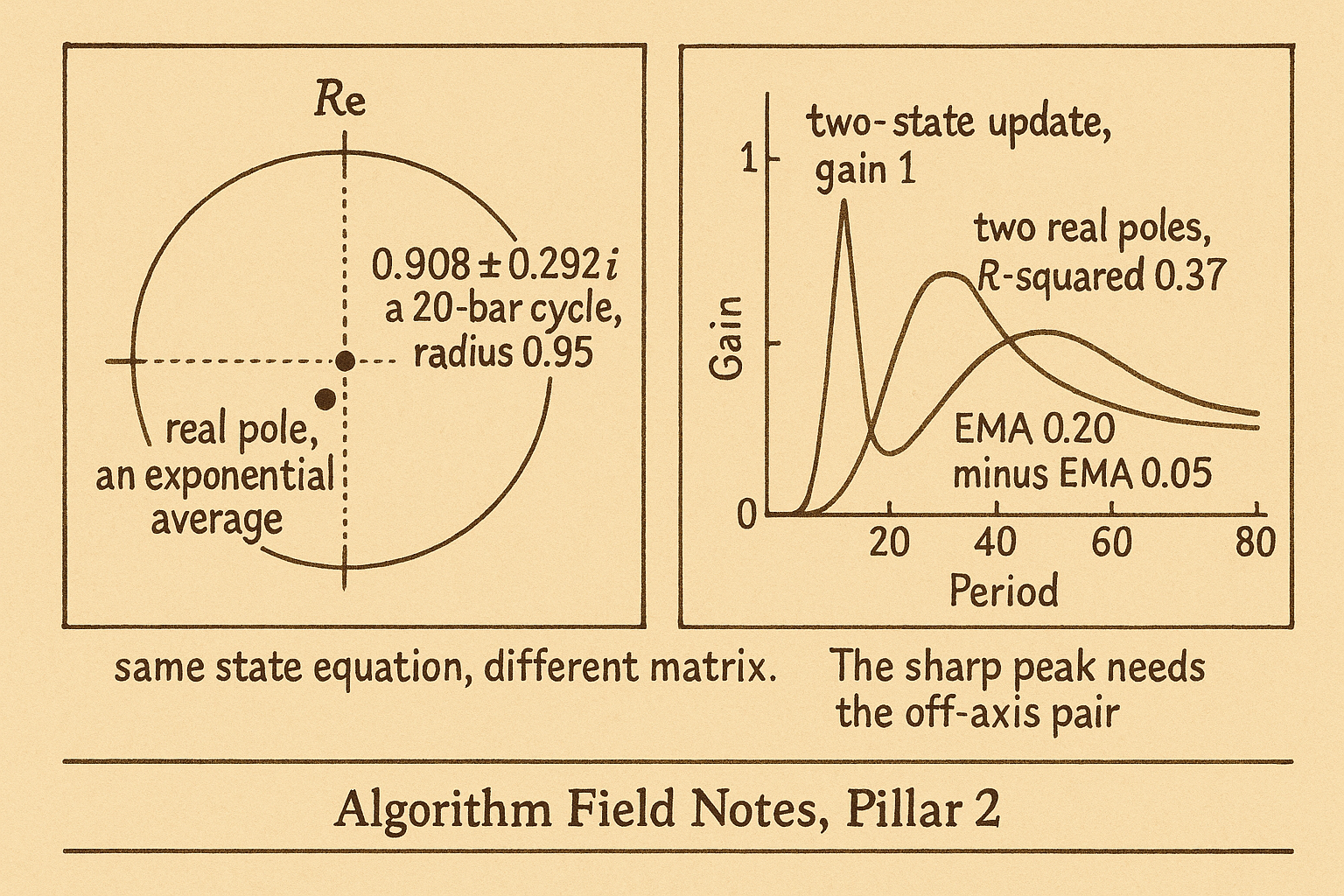
The top row is the recursion. The bottom row shifts the memory down by one bar. This is the discrete form of their state equation. The bottom-left entry is 1, so the two states are coupled, and the poles leave the real axis. The eigenvalues of that matrix are 0.908226 ± 0.291644 i. The radius is 0.953903, and the radius squared is 0.909931, which matches σ, the constant term of the characteristic polynomial. The angle of the pole is a 20.22-bar cycle. The zeros of the feed, the factor (1 - z inverse squared), sit at zero frequency and at the 2-bar cycle, so both of those gains are 0. The magnitude peak sits at period 20.00 with gain 1.000, and at that single frequency the output is real: phase is zero.
A pure sine checks it. Run a unit sine of period 20 through the recursion for 400 bars. Over the last cycle the largest gap between output and input is under 10 to the minus 7. The everlasting sine at the center period is copied. The envelope of a burst is not. Group delay is minus the slope of phase against angular frequency, in bars. At the center frequency that slope is 21.2 bars. The design rule that lands on the same figure: the quality factor Q is 1/δ, and the center group delay is Q times T over π.
$$ Q = \frac{1}{\delta}, \qquad \tau = \frac{Q \, T}{\pi} $$
Q is 1/0.3 = 3.333, and 3.333 · 20 / π is 21.22. The numerical slope was 21.20. Budget 21.2 bars for the envelope. The half-power points on the computed curve fall at 17.25 and 23.22 bars. The width is 5.97 bars, and 20 / 5.97 is a measured Q of 3.35, against the design value 3.33. The old article's table lists a lag of 9.5 bars for this same T and δ on daily SPX. The 9.5 and this 21.2 phase slope do not reconcile. Budget the phase slope. The source of the 9.5 may be measuring a different lag on SPX, or it may be wrong; the transfer function printed in that article gives 21.2.
Regressing the filter output on its own two lags and on the input difference recovers the three coefficients to six decimals, with an R-squared of 1. R-squared is one minus the residual variance divided by the label variance. Here the label was generated by the recursion, so the perfect fit is an identity check. The content of the check is that the identity is the state update above, three coefficients, all of order 1.
A diagonal fit peaks at 32 bars
CryptoMamba does not publish the trained state matrix, the input vector, or the readout. The layer below uses the scalar update they do print: two real decays, least squares on a known band-pass. The input is 20,000 draws of standard normal noise, generator seed 7. The label is the 20-bar band-pass of that same noise, bandwidth fraction 0.3. The first 400 bars are dropped. Each candidate decay a in a grid from 0.40 to 0.98, step 0.01, builds a state s_k = a s_{k-1} + u_k. Ordinary least squares, the readout weights that minimize squared error, picks the two gains. The search picks the pair of decays.
The winning decays are 0.81 and 0.82. The readout gains are 2.145 and -2.054. R-squared is 0.37. The gain curve of that frozen layer peaks at 32.1 bars, and the gain there, before any rescaling, is 0.286. Zero-frequency gain is 0.119, so a constant input still leaks. The 2-bar gain is 0.057. The two decays sit 0.01 apart, so the two states are nearly the same series and the fit manufactures a band-pass by subtracting them with large opposite weights.
Move the label. The same search against a 10-bar band-pass, same bandwidth fraction, returns decays 0.67 and 0.68, an R-squared of 0.31, and a peak at 16.4 bars. A noise label, unrelated to the input, returns an R-squared of 0.0001, with the decays shoved to 0.96 and 0.98 and readout gains near 0.01. The peak moves when the label's period moves, and it lands long of the label: 32 bars against a 20-bar target, 16 bars against a 10-bar target. Two real poles miss the resonator.
Adding diagonal states on a fixed grid, decays spaced from 0.50 to 0.98, creeps toward the target and spends the budget on cancellation. Four poles reach an R-squared of 0.60 and a peak at 25.4 bars, with a largest readout of 1.32. Eight poles reach an R-squared of 0.82 and a peak at 22.4 bars, with a largest readout of 184. Those readouts are a near-collinear cancellation. The 2 by 2 update in the previous section matches the same label with an R-squared of 1 and coefficients 0.045, 1.816, and -0.910.
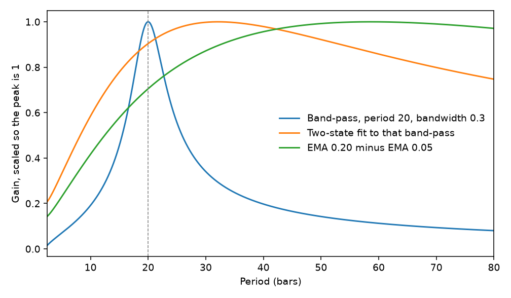
The blue curve is the band-pass, peaked on the dashed line at 20 bars. The orange curve is the two-real-pole fit. The green curve is the hand difference, α of 0.20 minus α of 0.05, topping out at 58.6 bars. Scaling each curve to its own peak is there so the locations can share an axis. The absolute peak gains are 1.00, 0.286, and 0.626.
Window length is a lag you can price
The same purchase shows up without any state matrix. The local average filtering objective in the old article "Fair Value as an Adaptive Low-Pass Filter: LAFO for Mean Reversion" scores a fitted line by the squared average residual inside a window of length K, then averages those squared window-means over the sample. The window operator there is a separate matrix from the state matrix A in the first section. Keep the two letters apart.
$$ \mathcal{L}(\hat{y}) = \frac{1}{T} \sum_{t=1}^{T} \left( \frac{1}{n_t} \sum_{k \in W_t} (y_k - \hat{y}_k) \right)^2 $$
W_t is the window ending at t, and n_t is how many bars it holds. K equal to 1 makes the inner average a single residual, and the loss is mean squared error: the fit chases every print. K equal to the sample length makes the loss care only about the average residual, and the line that zeros it is the sample mean. Their three-point check: residuals of +3, 0, and -3. At K of 1 the loss is the average of 9, 0, and 9, which is 6. At K of 3 the only window-mean is 0, and the loss is 0.
The lag of a symmetric window of length K is the symmetric-filter lag from the old article on lag, with the window length in the role of N.
$$ \mathrm{lag}(K) = \frac{K - 1}{2} $$
K of 1 costs 0 bars. K of 21 costs 10 bars. K equal to the sample costs half the sample, which is the global-mean pole of the loss above. Stretching K and lengthening a moving average are the same dial. You pay lag, and you buy a line that ignores the fast wiggle.
Wang's cubic smoother is that dial with the weights solved rather than set flat. On the Bybit BTC/USDT book, snapshots every 100 milliseconds, he fits a cubic on j from -10 to +10, twenty-one snapshots, by least squares, and replaces the window with the polynomial's value at j of 0. He writes the result as a fixed weighted sum and does not print the weights. Solving the normal equations gives them. They sum to 1.000, so a constant book is unchanged, and the weight on the current snapshot is 0.107551.
$$ \hat{v}_t = \sum_{j=-10}^{10} c_j \, v_{t+j}, \qquad c_0 = 0.107551, \qquad \sum_{j=-10}^{10} c_j = 1 $$
A flat book at 100 comes out at 100. The current snapshot is 10.8 percent of the smooth. The five snapshots after the print, j from 1 to 5, sum to 0.4479. At a 100-millisecond clock those five snapshots are the next 0.5 second, and the ten-bar symmetric lag is 1.0 second, sitting half in the future. The old article "Better Inputs Beat Deeper Nets: Crypto LOB Direction" measured this lookahead; the weights here match it. The gain of this weighted sum is 1 at long periods, 0.724 at 20 bars, 0.227 at 10 bars, and 0.103 at 5 bars. The 3 dB period, where the gain crosses 1 over the square root of 2, is 19.6 bars, which is 2.0 seconds. A 500-millisecond wiggle is a 5-bar cycle, and this smooth scales it by 0.10. The hit-rate jump in the next section is the score of a series that has already folded the next half-second into the feature.
A rejected order is a readout, and so is a filter
Albers, Cucuringu, Howison, and Shestopaloff have the clean case of a coefficient with nothing behind it in the book. On the Hyperliquid BTC-USD perpetual, September 2025, a post-only maker order that would cross the spread is rejected. The rejection never enters the book, never prints in the ordinary feed, and cannot move the mid. They count about 60,310 such rejections a minute, 86 percent of order submissions, on the order of 3.3 billion dollars of notional a minute. A rejected buy lines up with a later rise, and a rejected sell with a later fall, on 72.3 percent of the next price changes. The median wait to that change is about 2 seconds.
The regression they run first is the next 10-second midprice return, in basis points, on a signed indicator that is +1 for a rejected buy and -1 for a rejected sell. A basis point here is 0.01 percent of the mid.
$$ R_t = -0.1178 + 0.4242 \, \mathbf{1}_t^{\mathrm{rej}} $$
A rejected buy gives -0.1178 + 0.4242, which is 0.3064 basis points over the next 10 seconds. A rejected sell gives -0.1178 - 0.4242, which is -0.5420. The swing from sell to buy is 0.8484 basis points. The taker fee on that venue runs from 1.44 to 2.7 basis points. The cheapest fee is 1.44 / 0.3064 = 4.70 times the buy-side prediction. Leave the spread uncrossed on this coefficient.
Their comparative regression adds the top-of-book imbalance, a z-scored spread, the rejected-flow imbalance over the last 100 post-only submissions, and the imbalance of the post-only orders that did land. Imbalance is bid size minus ask size, divided by the sum. The spread z-score subtracts the day's mean and divides by the day's standard deviation.
$$ R_t = -0.1366 + 0.6224\,\mathrm{imb}_t + 0.0305\,\mathrm{Spread}_t + 0.1674\,\mathrm{imb}_t^{\mathrm{rej}} + 0.0705\,\mathrm{imb}_t^{\mathrm{open}} $$
Set the spread z-score to 0 and all three imbalances to +1. The predicted return is -0.1366 + 0.6224 + 0.1674 + 0.0705, which is 0.7237 basis points. Their prose says the predicted 10-second return, with an imbalance at its extreme, is at most a few tenths of a basis point. A single coefficient matches that phrase: the book imbalance alone, added to the intercept, is -0.1366 + 0.6224 = 0.4858. The sum of the three imbalance coefficients at +1 does not. It is 0.72 basis points. Keep both. Either figure sits under the 1.44 basis point taker fee, so the economic conclusion survives the looser sentence. The R-squared of this regression is 0.045. The univariate R-squared is 0.022. The association is precisely estimated, their standard errors are 0.0003, and it explains about 2 percent of 10-second return variance.
The single-order coefficient falls from 0.4242 to 0.1354 once the rejected-flow imbalance is in the regression, and that flow's own coefficient is 0.5415. In the full regression the book imbalance, 0.6224, is more than three times the rejected-flow coefficient, 0.1674, which is itself more than twice the open-order coefficient, 0.0705. The order that never landed is a weaker readout of a signal that also skews the visible book.
That is the same structure as the gain curve. The old article "No Filter Is Predictive: What Traders Misunderstand About Smoothing" stands: the transfer function has only non-positive powers of z, so no future bar enters the formula. What a squared-error fit changes is where the gain sits. On the synthetic layer the peak moved from 32 bars to 16 bars when the label period moved from 20 to 10, and a label with no shared band left an R-squared of 0.0001. The filter concentrates gain near the band the label occupies. Two real poles land long of that band. The rejected order concentrates a signal that was already in the information the trader acted on. Neither object inserts a new observation into the book.
The smoother moves the hit rate by more than the network
Look at the green bar in the Logit group, the rightmost cluster. That is logistic regression after Wang's cubic smooth, on the next 500 milliseconds of the Bybit book.
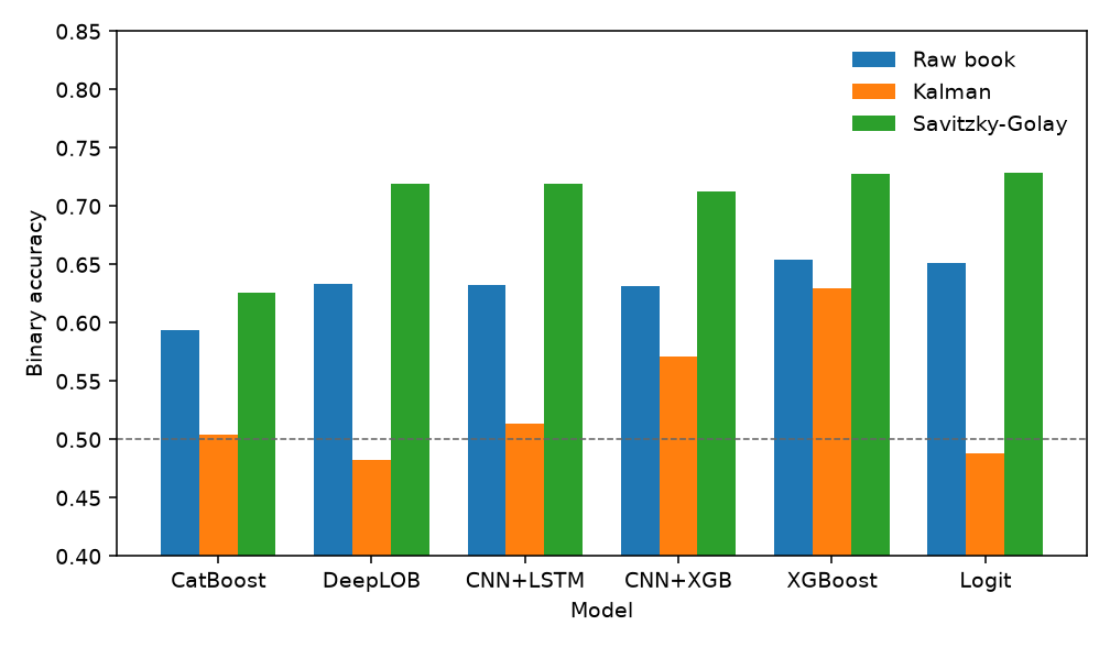
Logistic regression scores 0.7284 and DeepLOB, the convolutional net with a memory layer, scores 0.7189. Rounded to two decimals those are 0.73 and 0.72. The same logit on the raw book is 0.6517, so the smooth adds 0.08. XGBoost on that smooth is 0.73, CatBoost on it is 0.63, and the Kalman logit is 0.49, under the raw book's 0.65; every orange bar in the figure sits under its blue neighbor. The date is 30 January 2025, the clock is 100 milliseconds, and the five bars inside a 500-millisecond label already carry weight 0.45 in the smooth. The 1,000-millisecond smoothed XGBoost cell, the one later tied to 5,442 test rows, is 0.72.
On the daily Bitcoin tape the state-space comparison is a small gap between two state-space models. CryptoMamba's test root-mean-square error on the next close is 1713.0, against 1717.4 for S-Mamba, a difference of 4.40 dollars. With volume as an input the pair is 1598.1 against 1651.6. The old article on CryptoMamba already set the trading rule that turns 100 dollars into 262.78 next to holding Bitcoin over that one bull year, on about 350 test days and one random seed.
Freeze the layer and plot the gain
Plot gain against period, from 2 bars to 80, with B, C, and the step frozen, before you add parameters. If those three depend on the bar, freeze a quiet bar and a fast bar and plot both. Once a normalization and a linear layer wrap the update, the curve you can defend is the frozen update on its own.
When the cycle you trade is near 20 bars, use the 2 by 2 update. Gain at that period is 1, the 2-bar gain is 0, and the envelope is 21.2 bars late even though an everlasting sine at the center comes out in phase. The old article "Why Market Cycles Are Evanescent" is why you re-estimate a center of 20, or widen δ, on a window you are willing to defend. A two-real-pole substitute for this job peaked at 32 bars and left an R-squared of 0.37 on the label it was fitted to.
For a smooth you can run live, set the lag and take the exponential weight that prices it. A 10-bar lag wants α of 1/11, which is 0.0909, because (1 - α) / α then equals 10. The 21-point cubic needs ten snapshots that have not printed yet, so you can form it only after that second has arrived, and a 5-bar cycle is already scaled to a gain of 0.10. The causal Kalman smooth in the bar chart loses to the unsmoothed book.
Leave the rejected-order coefficient in the log. A predicted 0.31 basis points sits under the 1.44 basis point taker fee, and the authors note that their rejected-order feed arrives too late for the sub-second horizon they measure. The visible book imbalance, coefficient 0.62 in the same regression, is the larger readout of the same intent.
I am against replacing the two-line recursion with CryptoMamba's 136,000 parameters until a week you did not use to pick the poles shows the frozen layer peaking on the cycle you trade. They do not publish that matrix. The test tape is one year of one instrument.
KEY POINTS
- Discretize one pole before you treat a state-space model as a new indicator. A of -0.5 over one bar decays by 0.606531, and the zero-order-hold input weight is 0.786938.
- Audit a 20-bar band-pass by the sine it copies and by the envelope it delays. Gain at the center is 1, phase there is 0, and the group delay is 21.2 bars.
- Fit a two-real-pole layer to that band-pass and read the peak. The fit peaks at 32.1 bars with an R-squared of 0.37; a 10-bar label moves the peak to 16.4.
- Price the window with the symmetric lag. A 21-point cubic costs 10 bars, 1.0 second on a 100-millisecond book, and the five future snapshots inside that window carry weight 0.4479.
- Score the smoother before the network. On Wang's next-500-millisecond Bybit cell, logistic regression after the cubic scores 0.73 and DeepLOB scores 0.72.
References
- Band-Pass Filters: The Most Underused Tool in Technical Analysis
- State-Space Models for Price: CryptoMamba vs Transformers (Skeptical)
- The Trader's Guide to Low-Pass Filters
- The Hidden Cost of Every Moving Average: Lag
- The Frequency Response of Trading Indicators
- Fair Value as an Adaptive Low-Pass Filter: LAFO for Mean Reversion
- Better Inputs Beat Deeper Nets: Crypto LOB Direction
- No Filter Is Predictive: What Traders Misunderstand About Smoothing
- Why Market Cycles Are Evanescent
- CRYPTOMAMBA: LEVERAGING STATE SPACE MODELS FOR ACCURATE BITCOIN PRICE PREDICTION, Mohammad Shahab Sepehri, Asal Mehradfar, Mahdi Soltanolkotabi, and Salman Avestimehr
- The Price Impact of Nothing: Rejected Orders as Predictors of Future Returns, Jakob Albers, Mihai Cucuringu, Sam Howison, and Alexander Y. Shestopaloff
- Exploring Microstructural Dynamics in Cryptocurrency Limit Order Books: Better Inputs Matter More Than Stacking Another Hidden Layer, Haochuan (Kevin) Wang
A note on AI. The ideas, research, analysis, and conclusions in this article are my own. I use AI tools to help with editing and wordsmithing, because English is not my first language, and I am not shy about that. AI-generated ideas and AI-assisted writing are not the same thing: the first is empty slop from a generic prompt, the second is a tool for communicating years of real research more clearly. Judge the work by its substance, not by whether software helped polish the prose.