6.56 Fair Value as an Adaptive Low-Pass Filter: LAFO for Mean Reversion
Fair value is a low-pass filter with a dial, not a moving average. LAFO makes the cutoff explicit and neural filters turn corners faster than an EMA, but the headline Sharpe of 11 is pure in-sample.
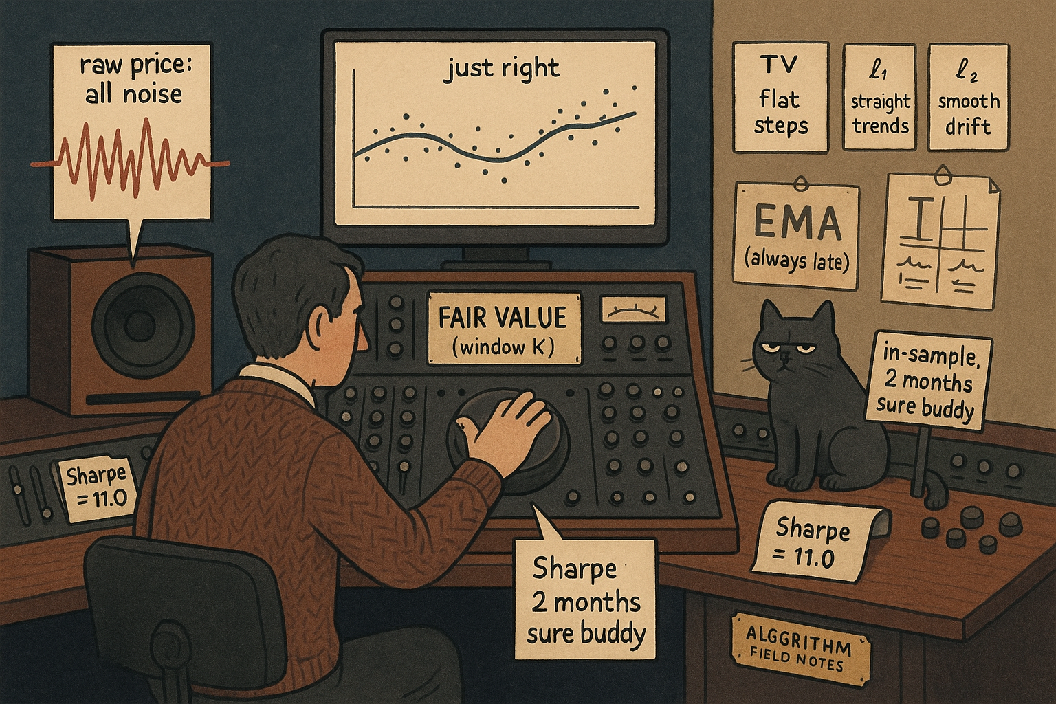
Every mean-reversion trade starts with a lie you tell yourself about where price "should" be. You call it fair value, you subtract it from the spot price, and you bet the gap closes. Most traders reach for a moving average and stop thinking. Xu, Firoozye, Koukorinis, Treleaven, and Zhu at UCL take the question seriously and reframe fair value as the output of a tunable low-pass filter, then train neural networks to produce it. The framework is clean and the math is honest. The trading results are a demo the authors themselves refuse to defend, and one of them is an in-sample 2-minute Sharpe of 11, which should make you laugh before it makes you curious.
The old article "Percentile-Rank Momentum With Hysteresis: Low-Churn Signals" fought the same enemy from the other side: a signal that flips too often bleeds you on costs, so you smooth it and add a deadband. This paper gives the smoothing a name, an objective function, and a dial. Fair value is a low-frequency component you extract from a noisy price; the only real decision is how much high-frequency noise to let through, and everything else follows from that.
The dial: one window that spans MSE to the global mean
The paper's core object is the local average filtering objective, LAFO. Instead of fitting the filtered line to every price point (which chases noise), it fits the average residual inside a sliding window of length K.
$$ \mathcal{L}_{\text{LAFO}}(\hat{y}) = \frac{1}{T} \sum_{t=1}^{T} \bar{e}_t^{\,2} = \frac{1}{T} \sum_{t=1}^{T} \left( \frac{1}{n_t} \sum_{k=a_t}^{b_t} (y_k - \hat{y}_k) \right)^2 = \frac{1}{T} \, \lVert A(\mathbf{y} - \hat{\mathbf{y}}) \rVert_2^2 $$
Read it in pieces. The term y minus y-hat is the residual, the gap between the real price and your fitted fair value. The inner sum averages that gap over the last K bars, so e-bar-t is the local average residual ending at time t. LAFO squares those local averages and averages them over the whole series. The matrix A is just the sliding-average operator that turns raw residuals into windowed ones, so the whole thing collapses to the squared length of A times the residual vector. Because A-transpose-A is positive semidefinite, the objective is convex, so it has a well-behaved minimum.
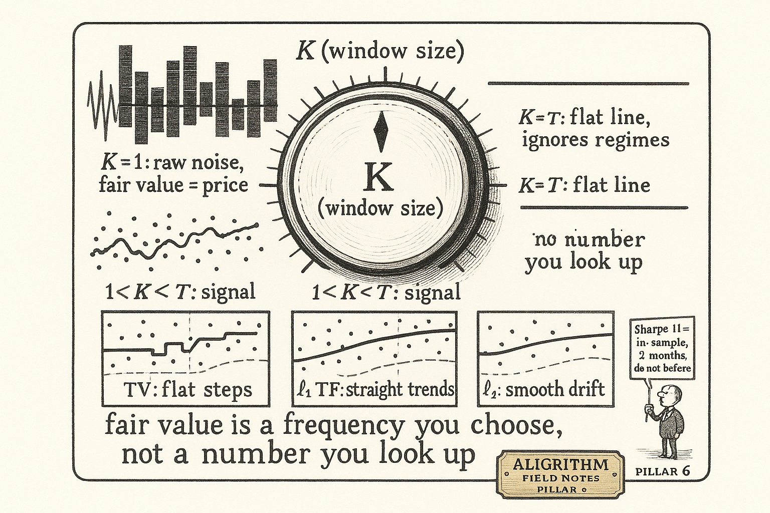
Work the window at its two extremes, because that is where the intuition lives. Set K equal to 1 and the window is a single bar: the local average residual is just the raw residual, A becomes the identity, and LAFO reduces to plain mean squared error, which fits every wiggle. Set K equal to T, the whole sample, and the objective only cares about the average of all residuals, so the best fit is a flat line at the global mean. A three-point series with residuals of plus 3, 0, and minus 3 has an MSE of 6 (the average of 9, 0, 9) at K equals 1, but a LAFO of 0 at K equals T because the residuals sum to zero. Same fit, opposite verdict. Every useful K sits between those poles, trading local responsiveness against smoothness.
$$ K = 1 \;\Rightarrow\; A = I \;\Rightarrow\; \text{standard MSE (fits all noise)} \qquad\qquad K = T \;\Rightarrow\; \text{rank}(W) = 1 \;\Rightarrow\; \text{global mean only} $$
That single knob is the whole pitch. Fair value is not a fixed recipe; it is a frequency cutoff, and K is where you set it. A Fourier analysis in the paper confirms the picture: larger K passes lower frequencies and kills more of the high-frequency chop.
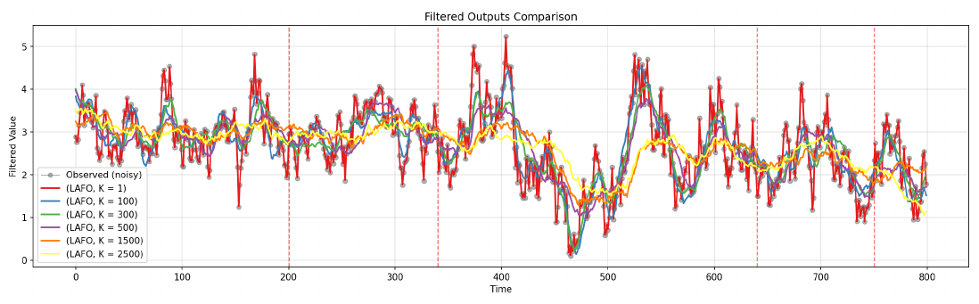
Look at the red line, K equals 1: it lies on top of the noise, useless as a fair value because it says price is always already at fair value. The yellow line, K equals 2500, barely moves, so it calls almost everything a deviation and would have you fading real regime shifts. The middle windows are the only ones that separate signal from noise, and picking one is the actual job.
Setting K without fooling yourself
The paper is candid that K is a choice, not a constant handed down by nature, and it offers three data-driven ways to set it. Match K to the expected regime length, near the median regime half-life, so the filter accentuates deviations on the horizon you actually trade. Or use the return autocorrelation: take K as the smallest lag where the absolute autocorrelation drops below a threshold like 0.1, which is the point past which recent moves stop predicting the next one. Or run rolling walk-forward cross-validation over a grid of K values (8, 16, 32, 64, 128, and so on) and let out-of-sample error pick.
Only the third method is honest for trading, and it is the one the paper skips in its actual backtest. The first two calibrate K to properties of the same sample you then trade, which is the in-sample bias the old article "State-Space Models for Price: CryptoMamba vs Transformers (Skeptical)" spent its whole length warning about. A cutoff frequency tuned on the data it filters will always look sharp in the picture and blurry in production.
The penalty picks the regime shape
The window controls how much you smooth. A penalty term controls the shape of what survives, and this is where the framework earns its keep over a moving average. Add one of three penalties on the differences of the filtered line.
$$ \text{TV: } \lambda \sum_{t=2}^{T} \lvert \hat{y}_t - \hat{y}_{t-1} \rvert \qquad \ell_1\text{ TF: } \lambda \sum_{t=3}^{T} \lvert \hat{y}_t - 2\hat{y}_{t-1} + \hat{y}_{t-2} \rvert \qquad \ell_2\text{: } \lambda \sum_{t=2}^{T} (\hat{y}_t - \hat{y}_{t-1})^2 $$
Each penalty punishes a different kind of movement. Total variation penalizes the sum of absolute first differences, the step sizes, so it drives most steps to exactly zero and leaves a piecewise-constant line that jumps only at genuine level breaks. The l1 trend-filtering penalty hits second differences, the changes in slope, so it produces a piecewise-linear line that bends only at a few regime transitions. The l2 penalty squares the first differences, which never forces anything to zero and instead spreads adjustment across every bar, giving a globally smooth curve. Lambda sets how hard each penalty pushes. Take three consecutive fair-value points at 100, 101, 100.5: the first difference is plus 1 then minus 0.5, and the second difference is minus 1.5, so TV pays 1.5 in penalty on the levels while l1 TF pays 1.5 on the single slope change. The choice of penalty is a bet on how the market's fair value actually moves: in flat steps, in straight trends, or in gentle drift.
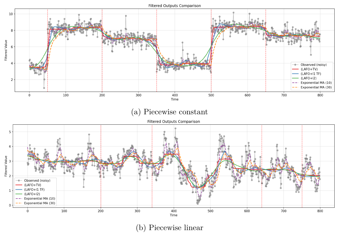
The comparison against exponential moving averages is the point of the figure. The dashed EMA lines round off every corner and arrive late at each regime break, which is exactly the lag that costs mean-reversion traders money when the "deviation" they are fading is really the fair value having moved. The l1 penalties turn corners on time. That is a real improvement over a moving average, and it is the honest contribution of the paper.
From filter to trade
Once you have a fair value, the strategy is mechanical. Measure the relative gap between spot and filter, and take a position against it.
$$ \delta_t = \frac{y_t - \hat{y}_t}{\hat{y}_t} \qquad w_t = \begin{cases} -\operatorname{sgn}(\delta_t)\,\min\{1,\ \alpha \max(0,\ \lvert \delta_t \rvert - \tau_{\text{entry}})\}, & \lvert \delta_t \rvert \geq \tau_{\text{entry}} \\ 0, & \lvert \delta_t \rvert < \tau_{\text{entry}} \end{cases} $$
Delta-t is the mispricing: how far spot sits above or below fair value, in percent. The position rule does nothing while the gap is inside a deadband of width tau-entry, then leans against the gap with size scaling up to a cap of 1. The minus-sign-of-delta means you short when price is above fair value and buy when it is below, the whole mean-reversion premise. Work it with the paper's settings, tau-entry of 0.0005 and alpha of 200. If spot is 5000.5 and fair value is 5000, then delta is 0.5 over 5000, which is 0.0001, below the 0.0005 band, so you stay flat. If spot is 5005, delta is 0.001, above the band; the position is alpha times (0.001 minus 0.0005), which is 200 times 0.0005, so 0.1, a tenth of full size short. The deadband is the same anti-churn hysteresis idea as the old article "Percentile-Rank Momentum With Hysteresis: Low-Churn Signals," here applied to a reversion signal instead of a momentum one.
The results, and why the Sharpe of 11 is a warning
The paper trades this on 2-minute S&P 500 data over two months, feeds every model the same LAFO window (K equals 80) and the same trading parameters, and charges 3 basis points per unit of turnover. The neural filters beat the moving averages by a wide margin.
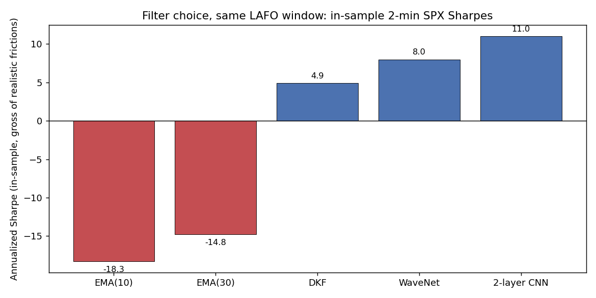
The 2-layer CNN posts an annualized Sharpe of 11.049, a hit rate of 0.479, and a Sortino of 39.13. WaveNet lands 8.005, the deep Kalman filter 4.920. Both exponential moving averages are deeply negative: EMA(10) at minus 18.265, EMA(30) at minus 14.761. Read literally, a two-layer convolutional net turned the same fair-value framework that sinks a moving average into a Sharpe north of 11.
Do not read it literally. A Sharpe of 11 on two months of 2-minute bars is not an edge, it is a flashing in-sample-overfit light. The authors say so themselves, in plain text: the models are "applied without systematic parameter calibration," the study is "primarily methodological," and out-of-sample evaluation "should be addressed in a separate paper." There is no walk-forward, no retraining, no second dataset. The window K, the penalty lambda, the entry band, and the position scale were all set on the same two months that produced the Sharpe. The negative moving-average numbers are just as suspect in the other direction: a fixed EMA lag fed the same tiny deadband on the same noisy series is being set up to lose. What the table actually shows is that a flexible filter fits two months of 2-minute SPX better than a rigid one. That is unsurprising and not tradable.
The one durable finding hides in the same table. Model complexity did not help. The small 2-layer CNN beat the heavier WaveNet and the deep Kalman filter, and the paper attributes this to the larger models being data-hungry and unstable on a 6,000-sample set. That rhymes with the old article "State-Space Models for Price: CryptoMamba vs Transformers (Skeptical)": on short financial samples, the fancy architecture usually loses to the simple one, and the burden of proof sits with anyone claiming otherwise.
What to keep and what to bin
Keep the framing. Fair value as a low-pass filter with an explicit cutoff is a genuinely better mental model than "use the 20-day average," because it forces you to name the frequency you are separating and to choose a penalty that matches how you think fair value moves. Keep the penalty menu: TV for level regimes, l1 trend filtering for trending regimes, l2 for smooth drift, each with a lag advantage over an EMA at the regime breaks. Keep the deadband trade rule; it is the same low-churn discipline that survives contact with transaction costs.
Bin the performance numbers. Every Sharpe in the table is in-sample, single-asset, two months, with all filter and trade parameters fitted on the test window and no out-of-sample check, which is why the authors label it a demo. Treat the 11.0 as a stress test of your own credulity, not as evidence. Before any of this touches capital it needs the full gauntlet: walk-forward K selection, purged cross-validation, multiple assets, and a permutation test on the reversion signal. The paper builds a clean pipe and honestly declines to certify the water. That honesty is worth more than the headline.
Where this connects
This is the smoothing engine under the old article "Percentile-Rank Momentum With Hysteresis: Low-Churn Signals." That piece built a low-churn signal by ranking, then adding a deadband so the position stops flickering; here the deadband reappears as tau-entry, and the ranking-versus-raw-price question becomes a filtering-frequency question. Both are fights against the same tax: a signal that reacts to every tick pays the spread to death, so you decide, on purpose, how much of the high-frequency world to ignore.
It also belongs next to the old article "Wave Velocity and Acceleration: Reading When the Market Runs Out of Gas," which chased the same grail from digital signal processing: reading a turn early, without the lag a moving average adds. That piece got its early read from the exact derivative of a local sine model; LAFO gets its from penalty structure. The moving average lags because it is a fixed low-pass filter with no penalty; the l1 penalties in LAFO cut the lag at regime breaks precisely because they allow sharp, sparse changes instead of spreading every adjustment across the window. Same target, a filter that is smooth in the quiet and fast at the breaks, reached with an explicit objective instead of a clever recursion, and both inherit the same fragility when the model of the underlying shape is wrong.
And the skepticism is borrowed straight from the old article "State-Space Models for Price: CryptoMamba vs Transformers (Skeptical)." A tiny out-of-sample window, a single asset, and a headline number too good to be true are the exact tells that piece flagged. The 2-layer CNN beating WaveNet and the Kalman filter is the same lesson twice: on short, noisy financial data, complexity is a liability until proven otherwise, and a two-month Sharpe of 11 is a hypothesis about overfitting, not a strategy.
KEY POINTS
- Fair value is better modeled as the output of a tunable low-pass filter than as a fixed moving average. LAFO fits the average residual inside a window of length K, so K is an explicit dial for how much high-frequency noise you let through.
- The window spans the two things traders already do badly: K equal to 1 is plain MSE that fits all noise (fair value equals price, useless), and K equal to the whole sample is a flat global mean that ignores regimes. The tradable filter lives strictly between.
- The penalty sets the regime shape. Total variation gives flat steps, l1 trend filtering gives straight trends, l2 gives smooth drift, and all three turn corners at regime breaks faster than an exponential moving average, which lags.
- Trading is a deadband rule on the relative gap between spot and filter: stay flat inside tau-entry, then lean against the gap up to a size cap. This is the same anti-churn hysteresis that keeps costs from eating a reversion signal.
- On 2-minute SPX over two months at 3 bps cost, the 2-layer CNN posted an in-sample Sharpe of 11.0, WaveNet 8.0, the deep Kalman filter 4.9, while EMA(10) and EMA(30) were deeply negative at minus 18.3 and minus 14.8.
- Do not trust those Sharpes. The authors state the study is methodological, with no calibration and no out-of-sample test, and all parameters were fitted on the same two months. A Sharpe of 11 on 2-minute bars is an overfit tell, not an edge.
- The one durable result: the small CNN beat the larger WaveNet and Kalman models, because complex architectures are data-hungry and unstable on a 6,000-sample set. On short financial data, simple filters win until proven otherwise.
A note on AI. The ideas, research, analysis, and conclusions in this article are my own. I use AI tools to help with editing and wordsmithing, because English is not my first language, and I am not shy about that. AI-generated ideas and AI-assisted writing are not the same thing: the first is empty slop from a generic prompt, the second is a tool for communicating years of real research more clearly. Judge the work by its substance, not by whether software helped polish the prose.