5.51 Better Inputs Beat Deeper Nets: Crypto LOB Direction

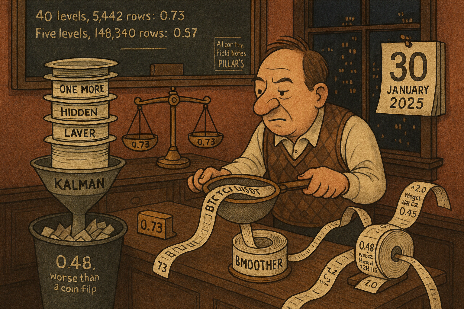
Wang reports logistic regression at 0.7284 binary accuracy on the next 500 milliseconds of the Bybit BTC/USDT limit order book, XGBoost, a gradient-boosted tree, at 0.7281, and DeepLOB, the convolutional network with a memory layer from Zhang, Zohren, and Roberts, at 0.7189. All three use a 40-level book smoothed with a Savitzky-Golay filter, a local cubic average. Under a Kalman filter, a causal running estimate, that same DeepLOB score is 0.4825, below a coin flip and below the raw-book score of 0.6333. His largest printed test, 148,340 rows at five levels, scores 0.5732 for XGBoost. The date is 2025-01-30, the clock is 100 milliseconds, and the smoother, as written, uses prices up to one second ahead.

What this actually is

You quote BTC/USDT on Bybit. A fresh book arrives every 100 milliseconds, and a one-lot quote can show up and vanish inside that gap, so the mid-price prints a move with no trade behind it. You want a single bit, up or down, over the next 500 milliseconds to the next second, so you can lean a bid or an offer before that flicker dies.

Wang smooths the snapshots and has a linear classifier, a tree model, and several neural networks call that same bit.

Picture a harbor radio bolted to the wall beside a pile driver. Extra circuitry in the receiver still picks up the hammer. Shutting the window removes more of the hammer than any new circuit does.

His smoother is that window, and it faces forward: the value dated now mixes in prices from up to one second ahead, the same second he scores as a forecast. The Kalman filter faces backward and loses to the unsmoothed book on his table. If a backward-looking smooth still left the linear classifier level with the deep network on a second day, you would spend the research week on the smoother, the up/down cutoff, and the rule for dropping thin books, and you would ship the linear score as a quoting skew. Crossing the spread needs the size of the move, and he publishes the sign. Taking the published 0.7284 as a live hit rate means leaning on a feature that can see its own label, scored on the snapshots that still had 40 price levels, from a file he dates to one day.

Four inputs you can compute from one book

The question is what a logistic model can see before anyone stacks a hidden layer. Kercheval and Zhang ran hand-built book features of this kind through a linear classifier on equity limit-order books. Wang builds four inputs from the top of the book. The mid is the average of the best ask and the best bid. The top-of-book imbalance is the bid size minus the ask size, divided by the sum of the two sizes. The five-level version does the same with the summed sizes. The weighted mid change is a blend of recent mid changes at the first three depths, with weights proportional to one over the depth index and scaled so they sum to one.

$$ m_{t-1} = \frac{a_{t-1}^{1} + b_{t-1}^{1}}{2} $$ $$ I_t^{1} = \frac{Q_{t,1}^{b} - Q_{t,1}^{a}}{Q_{t,1}^{b} + Q_{t,1}^{a}}, \qquad I_t^{5} = \frac{\sum_{i=1}^{5} Q_{t,i}^{b} - \sum_{i=1}^{5} Q_{t,i}^{a}}{\sum_{i=1}^{5} Q_{t,i}^{b} + \sum_{i=1}^{5} Q_{t,i}^{a}} $$ $$ \Delta m_t^{w} = \sum_{i=1}^{3} w_i \left(m_t^{i} - m_{t-1}^{i}\right), \qquad w_i \propto \frac{1}{i}, \qquad \sum_{i=1}^{3} w_i = 1 $$

Read it as: a and b are ask and bid prices in USDT, Q is size in BTC, m is a mid in USDT, I is a dimensionless ratio between minus one and plus one, and delta-m is a USDT change. The superscripts and the index i are depth, starting at the touch. Wang writes the level mid inside the weighted change without a separate definition; the reading here is the mid at that depth.

Worked snapshot, invented so the arithmetic is visible, in the same 103,700 USDT neighborhood as his filter chart. Best ask 103,710, best bid 103,700, so the mid is 103,705 USDT. Touch sizes 12 BTC bid and 4 BTC ask: imbalance is (12 minus 4) over (12 plus 4), which is 8/16, so 0.50. Five levels of bids 12, 8, 5, 3, 2 sum to 30 BTC. Five levels of asks 4, 6, 8, 10, 12 sum to 40 BTC. Five-level imbalance is (30 minus 40) over 70, which is minus 1/7, about minus 0.143. The touch says the bid is heavy. The next four levels say the offer is stacked behind it. Both features belong in the model because they disagree on this book.

Weights proportional to 1, 1/2, and 1/3, then normalized, are 6/11, 3/11, and 2/11. Suppose the three depth mids changed by plus 1.0, plus 0.4, and minus 0.2 USDT. The weighted change is (6/11)(1) plus (3/11)(0.4) plus (2/11)(minus 0.2), which is 6.8/11, or 0.618 USDT.

His introduction sends these inputs to logistic regression and to XGBoost. His methods section then says the XGBoost run flattens the whole snapshot, T past snapshots by F book columns, into one long vector. The tables never say which of those two recipes produced a cell. He does not reconcile them.

The old article "Reconstructing the Order Book from Incremental Deltas" is the step this file skips. Bybit hands him a snapshot, top 200 bids and asks, with a NaN where a level is missing. He drops any row that lacks the depth he asked for. A missing level 40 is often a thin book, and deleting the row is a sample choice, which shows up later as a test set of 5,442 instead of 20,000.

The smooth value dated now uses the next second

The question is whether the accuracy jump is a filter a live book can run. Before the model, he runs one of two smoothers over each series. The Savitzky-Golay smoother, Savitzky and Golay's 1964 local-polynomial fit, places a cubic on a centered window of 21 snapshots, j from minus 10 to plus 10, by least squares, then replaces the window with a fixed weighted average. At a 100-millisecond clock, 10 snapshots is 1.0 second.

$$ \min_{a_0,a_1,a_2,a_3} \sum_{j=-10}^{10} \left[ v_{t+j} - (a_0 + a_1 j + a_2 j^2 + a_3 j^3) \right]^2 $$ $$ \hat{v}_t = \sum_{j=-10}^{10} c_j \, v_{t+j} $$

Read it as: v is the raw series in USDT (a mid, or a size, or a price), j is a snapshot offset with no unit other than "100 milliseconds each," a0 through a3 are the cubic's coefficients, c sub j is the dimensionless weight you get once that least-squares problem is solved for this fixed window, and v-hat is the smoothed value in the same unit as v. The weights sum to 1. They are symmetric. Wang's equation (6) is the normal equation behind c; the convolution is the object you would code.

Solving that window gives a center weight of 0.1076. The weight one snapshot ahead, 100 milliseconds, is 0.1059, almost the same as the weight on now. The five future snapshots inside a 500-millisecond label carry a combined weight of 0.4479. The current print carries 0.1076. The smoothed "price" dated now is more the next half-second than it is the print in front of you. The weight at plus 10 snapshots is minus 0.0559, a negative lobe at the rim of the window, so the leak is signed, and a model can flip it.

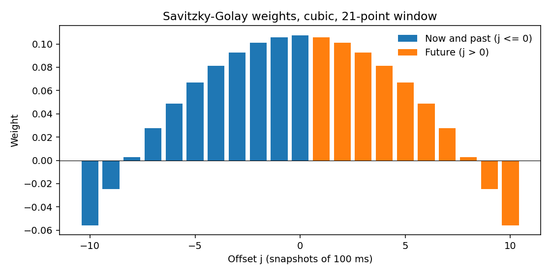
Worked check. Twenty-one prints, all 103,700 USDT, smooth to 103,700 because the weights sum to 1. Lift only the snapshot 100 milliseconds ahead by 10 USDT, to 103,710. The smoothed value dated now becomes 103,700 plus 10 times 0.1059, which is 103,701.06 USDT. Lift only the snapshot 1.0 second ahead by that same 10 USDT and the smoothed value dated now becomes 103,700 plus 10 times minus 0.0559, which is 103,699.44 USDT. A 500-millisecond label is the sign of the mid five snapshots ahead. Those five snapshots are inside the feature. A 1,000-millisecond label's endpoint is the negative lobe. He publishes no lagged window, the causal version that uses j from minus 20 to 0 and dates the result at the right edge. That lag is 1.0 second. On a 1-second forecast the lagged smooth arrives as the horizon expires.

The Kalman filter in his equations (8) through (10) is causal. A latent price does a random walk with process variance Q. You observe it plus noise of variance R. The gain, the updated estimate, and the updated variance are a recursion that uses the current print and the previous estimate.

$$ K_t = \frac{P_{t-1} + Q}{P_{t-1} + Q + R} $$ $$ \hat{x}_t = \hat{x}_{t-1} + K_t \left(v_t - \hat{x}_{t-1}\right), \qquad P_t = (1 - K_t)\,(P_{t-1} + Q) $$

Read it as: x-hat is the estimated price in USDT, v is the observed print in USDT, Q and R and P are variances in USDT squared, and K is a dimensionless gain between 0 and 1. K is the fraction of the surprise you accept. Large R, a print you have declared noisy, keeps K small and the estimate glued to its past.

He does not print Q or R. Illustration of the update, not his fit: Q = 0.25, R = 1, previous variance P = 0.25, all in USDT squared. The gain is (0.25 plus 0.25) over (0.25 plus 0.25 plus 1), which is 0.5/1.5, or 1/3. Previous estimate 103,700, new mid 103,706. The update is 103,700 plus (1/3) times 6, which is 103,702 USDT. The new variance is (2/3) times 0.5, which is 1/3. Two-thirds of a 6 USDT jump is thrown away. Do that on every real move and the series lags the book the forecast is aimed at. He says the variances were grid-searched on a small sample and then frozen. The text points this filter at "Wu et al., 2011," and the bibliography's Wu paper is a 2021 note on perturbed books. The recursion above is what he wrote down.

On that 200-second slice the two smoothers are hard to tell apart by eye. The accuracy table is where they split. Visual smoothness is a bad referee.

Up, down, and a flat band he never sizes

The question is what the hit rate is measured against. Binary labels are up or down. Ternary labels add a flat class inside a band of half-width epsilon around a zero return. He says he tunes epsilon, following Sirignano and Cont, so the three classes have about equal counts, and he reweights the loss by inverse frequency. He never prints epsilon, and the horizon tables never print the class counts.

A balanced coin flip is 0.50 on the binary task and 1/3 on the ternary task. At the 500-millisecond, 40-level, Savitzky-Golay cell, logistic regression's 0.7284 sits 0.2284 above 0.50. Its ternary score of 0.5434 sits 0.2101 above 1/3. The ternary number looks worse and the lift over a dumb baseline is in the same range. At 100 milliseconds on a 5-level book the binary scores sit between 0.5271 and 0.5338, a lift of about three points over 0.50, and the best ternary score is DeepLOB at 0.4281, a lift of 0.0948 over 1/3. Short horizon, thin book, small edge. The 0.73 does not live there.

He quotes logistic regression at 48 to 64 percent on the FI-2010 equity benchmark, depending on horizon. That range is his literature summary, tied to the Ntakaris dataset paper. It is a different market, a different clock, and a vendor-cleaned book. Read 0.73 against that yardstick with the sample attached: one date, and the smoother described above.

Eight points from the filter, one point from the network

Hold the filter fixed and the remaining question is the gap across models. Same 80,000 training rows and a nominal 20,000-row test, one snapshot of history (his T equals 1), six models. DeepLOB here is three convolutional blocks and an LSTM of 64 units, a recurrent layer that carries a state across snapshots. The simpler net is one convolutional layer and a bidirectional LSTM of 32 units. CNN plus CatBoost, which the table header shortens to CatBoost, is the Bileki pipeline: two convolutional layers, a 64-dimensional embedding, then a boosted tree. XGBoost is the tree on its own. Logistic regression is the linear score.

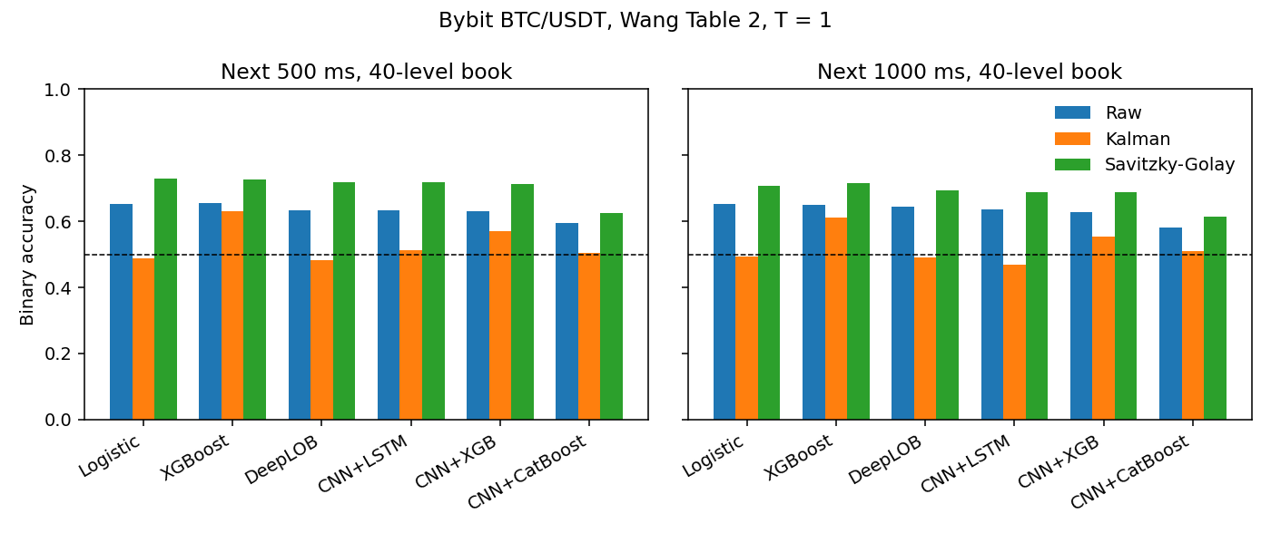
At 500 milliseconds, Savitzky-Golay, the order is logistic regression 0.7284, XGBoost 0.7281, DeepLOB 0.7189, the simpler net 0.7189, CNN plus XGBoost 0.7130, CNN plus CatBoost 0.6260. Logistic regression minus DeepLOB is 0.0095. Logistic regression minus CNN plus CatBoost is 0.1024. The plain tree and the linear score tie. The convolutional embedding handed to CatBoost gives back ten points against the tree that saw the snapshot without that embedding.

The filter moves the score by more than the model does. Logistic regression goes from 0.6517 on the raw book to 0.7284 after Savitzky-Golay, a gain of 0.0767, and to 0.4882 under Kalman, a drop of 0.1635. DeepLOB goes from 0.6333 raw to 0.7189 smoothed, a gain of 0.0856, and to 0.4825 under Kalman, a drop of 0.1508. XGBoost on the same Kalman book is 0.6301 against a raw 0.6542, a drop of 0.0241. Every binary cell and every ternary cell in the three horizon blocks is lower under Kalman than on the raw book. The damage is a couple of points for the plain tree and fifteen points for the linear model and for DeepLOB. On the raw 500-millisecond book, before any smoother, XGBoost at 0.6542 and logistic regression at 0.6517 already lead DeepLOB at 0.6333. Smoothing lifts the net by more than it lifts the logit, and the logit is still ahead.

At 1,000 milliseconds the smoothed order is XGBoost 0.7150, logistic regression 0.7089, DeepLOB 0.6947, CNN plus CatBoost 0.6140. XGBoost minus DeepLOB is 0.0203. He calls this a 1 to 2 percent edge for the simpler models. Read it as 1 to 2 percentage points, and read it against the nets, because CNN plus CatBoost is ten points back (0.7150 minus 0.6140 is 0.1010). The worst Kalman cell in the binary table is the simpler net at 1,000 milliseconds, 0.4680, against 0.6372 on the raw book.

The 0.0095 gap needs a noise scale. He prints two candidate test sizes and attaches neither to the 0.7284 cell. The 0.7150 cell, which is the smoothed XGBoost score at 1,000 milliseconds, is the one he later pairs with a support of 5,442.

$$ SE = \sqrt{\frac{p\,(1-p)}{n}} $$

Read it as: p is an accuracy between 0 and 1, n is the number of test snapshots, and SE is the sampling wobble of that accuracy in the same units. Worked at the headline accuracy, borrowing the 5,442-row support from the sister cell: p = 0.7284, so p times (1 minus p) is 0.19783, divided by 5,442 is 0.00003635, and the square root is 0.00603. The 0.0095 gap is 1.6 of those wobbles. Borrow the 20,000-row test he names in the section header and the wobble falls to 0.00315, so the same gap is 3.0 wobbles. The ten-point gap against CNN plus CatBoost survives either sample size. The one-point gap against DeepLOB is small if the test is the 5,442-row book.

Two confounders sit in the table headers. The 100-millisecond block is a 5-level book. The 500- and 1,000-millisecond blocks are 40-level books. A jump from 0.53 to 0.73 is a jump in horizon and a jump in depth at the same time. He calls the cells accuracy in the prose. In the paper, the section before the tables defines the F1 score, the harmonic mean of precision and recall, and the table header names no unit. The 0.7150 match with the later accuracy column is why these cells are accuracies.

A full book is a smaller sample

The question is whether 40 levels predict better, or whether a full book is an easier hour. He keeps the Savitzky-Golay smooth and XGBoost, drops any snapshot that lacks the k-th level, and lets k run from 40 down to 5. The accuracy he dissects here is 0.7150, the 1,000-millisecond cell, not the 0.7284 maximum of the binary table.

At 40 levels the accuracy is 0.7150, the two class F1 scores are 0.7115 and 0.7184, and the test support is 5,442. The average of those two F1 scores is 0.71495, which matches 0.7150 to rounding, the pattern of near-equal class counts. At 10 levels the accuracy is 0.5837 on 17,471 rows. At 5 levels it is 0.5797 on 18,336 rows. From 40 levels to 10, accuracy drops by 0.1313 and the test set more than triples. From 10 levels to 5, accuracy drops by 0.0040, inside the 0.006 wobble above, and the test set grows by 865 rows.

He says he trains on 80,000 and tests on 20,000. Against that 20,000, a 40-level requirement keeps 5,442 rows, 27.2 percent, and a 5-level requirement keeps 18,336, 91.7 percent. Levels 11 through 40 are where his number moves. He does not separate "those levels carry signal" from "hours with a full 40-level book are easier." A quoter who abstains when level 40 is empty posts 0.715 and trades 27 percent of the snapshots. A quoter who always trades posts something near 0.58. Those are different jobs, and the second one is the one a 24-hour book will hand you.

The old article "An Open L4 Order Book: What Hyperliquid Data Unlocks" is the feed that would label the flicker instead of smoothing it. A 100-millisecond snapshot cannot show a cancel that lived 30 milliseconds. It shows a mid that twitched. He reaches for a smoother because the file stored pictures, not the cancels between them.

Two points for ten snapshots

The question is what a longer lookback buys once the model is already simple. He switches to 1,000,000 snapshots at five levels, Savitzky-Golay, and predicts the mid change over the next 1,000 milliseconds from either one snapshot or ten. Ten snapshots cover 0.9 seconds from the first to the last; he calls that a second. XGBoost at T equals 1 scores 0.5732, with class F1 scores 0.5757 and 0.5707 whose average is the accuracy, on supports 73,953 and 74,387. That sum is 148,340 rows, 74.2 percent of a 200,000-row test, which he calls 75 percent. At T equals 10 the score is 0.5949. Logistic regression goes from 0.5551 to 0.5716. Gains of 0.0217 and 0.0165. He calls that about a 2 percent accuracy gain. Training time on an M2 laptop, for the million rows, goes from 1 minute 36 seconds to 7 minutes 4 seconds for XGBoost (4.4 times) and from 1 minute 11 seconds to 9 minutes 13 seconds for logistic regression (7.8 times).

His sentence places the T-equals-10 label one second after the sequence starts. A causal window of ten snapshots ends 0.9 seconds after it starts, so the label endpoint is 100 milliseconds past the last input. If the window is aligned the other way, most of the label path sits inside the input. He does not draw the alignment. A two-point gain is small for a feature that contained the answer, and it is the sort of gain extra history often produces. The million-row experiment is also the one that stays near 0.57, in line with the 0.5797 he got at five levels on the shorter file. The 0.73 does not reappear once the book is five levels deep and the test has 148,340 rows.

One date, no markout, no causal rerun

The question is what can go to a live quote. Section 3 says the study is the single day 2025-01-30. The conclusion says the main tables use about 100,000 snapshots, which at 100 milliseconds is 10,000 seconds, 166.7 minutes, and he writes about 166 minutes. That is a slice of the day, 11.6 percent of the 864,000 slots in 24 hours, if the grid is full. The million-row run is 100,000 seconds, 27.8 hours, and he writes about 28 hours. One UTC day cannot hold it. Either the file crosses midnight, or the grid has gaps and the "28 hours" is a count of slots rather than a clock, or the single-day sentence is too strong. He writes both. Neither sentence repairs the other.

He also never says the 80/20 split is chronological. "The first 100,000 snapshots" is a time prefix. The split inside it could be shuffled. On a 100-millisecond book a shuffled row shares its neighbors with the other side. Add the centered smoother, which already mixes ten future snapshots into every row, and a random split is a second leak on top of a first. Undescribed, so unproven. The centered window is proven from the summation limits.

The abstract says the models are compared on latency. The only clock in the results is training time for two models on one laptop. The remark about a network that hits 80 percent and takes two seconds to forecast the next one second is a hypothetical. His best printed cell is 0.7284, and he does not time the forward pass.

He prints no PnL, no spread, no fee, and no markout. A markout is the mid change over a fixed horizon after a fill, the number that says whether the fills were toxic. A sign hit rate has no PnL until the move clears the spread, and he never prints the move. Use the bit as a skew on a quote that was already going out. It becomes a trade after the markout clears the fee. He stops at the bit.

The old article "Does Complexity Actually Help? The Virtue-of-Complexity Autopsy" found the same shape on equity returns: once the comparison was specified, a plain ridge sat ahead of the high-order feature model. Here a linear score sits ahead of DeepLOB by a point, on a book that was smoothed with a window into its own label, on one date. The part worth keeping is the ranking of the filters. The 0.73 cell is a 40-level book on the short file. The large five-level test scores 0.57. The part to rerun, before anyone skews a live BTC quote, is a backward-looking window, a printed epsilon, a chronological split, and a second day.

KEY POINTS

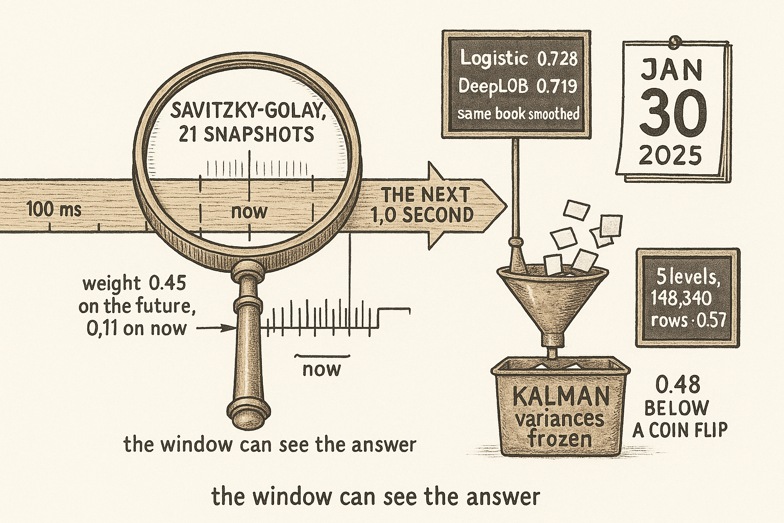
• On Bybit BTC/USDT, 100-millisecond snapshots, Wang's best binary cell is logistic regression at 0.7284 for the next 500 milliseconds, on a Savitzky-Golay smoothed 40-level book. XGBoost is 0.7281. DeepLOB is 0.7189. The gap over DeepLOB is about one percentage point.
• The same DeepLOB score is 0.6333 on the raw book and 0.4825 under his Kalman filter. Logistic regression falls from 0.6517 raw to 0.4882 under Kalman. Every binary cell and every ternary cell in the horizon tables is worse under Kalman than on the raw book. XGBoost loses only 0.024 on that 500-millisecond Kalman swap.
• The Savitzky-Golay window he specifies is a centered cubic on 21 snapshots. The five future snapshots inside a 500-millisecond label carry combined weight 0.4479. The current print carries 0.1076. He publishes no lagged, causal rerun. The Kalman recursion he writes is causal, and it loses to the raw book.
• Requiring 40 complete levels leaves 5,442 test rows at accuracy 0.7150. Five levels leaves 18,336 rows at 0.5797. Almost all of that drop happens between 40 and 10 levels (0.7150 to 0.5837). The 100-millisecond block is a 5-level book, so the horizon table mixes horizon with depth.
• The only experiment with 148,340 printed test rows is the five-level run: XGBoost 0.5732 at one snapshot and 0.5949 at ten, logistic regression 0.5551 and 0.5716. Training those on an M2 takes from 1 minute 11 seconds to 9 minutes 13 seconds. That is training time, not a forward-pass latency, and he never reports a PnL, a spread, or a markout.
• The main tables are about 100,000 snapshots, 166.7 minutes of 2025-01-30. The million-row run is 27.8 hours and does not fit in that single date as he also states it. The 80/20 split is not described as chronological. Treat 0.7284 as an upper bound from a smoother that can see its label, not as a live quoting edge.

References

• Modelling high-frequency limit order book dynamics with support vector machines, Kercheval and Zhang (2015)
• Benchmark dataset for mid-price forecasting of limit order book data with machine learning methods, Ntakaris, Magris, Kanniainen, Gabbouj, and Iosifidis (2018)
• DeepLOB: Deep Convolutional Neural Networks for Limit Order Books, Zhang, Zohren, and Roberts (2019)
• Universal features of price formation in financial markets: perspectives from deep learning, Sirignano and Cont (2019)
• Smoothing and Differentiation of Data by Simplified Least Squares Procedures, Savitzky and Golay (1964)
• Order book mid-price movement inference by CatBoost classifier from convolutional feature maps, Bileki, Barboza, Silva, and Bonato (2022)
• Exploring Microstructural Dynamics in Cryptocurrency Limit Order Books: Better Inputs Matter More Than Stacking Another Hidden Layer, Haochuan (Kevin) Wang

A note on AI. The ideas, research, analysis, and conclusions in this article are my own. I use AI tools to help with editing and wordsmithing, because English is not my first language, and I am not shy about that. AI-generated ideas and AI-assisted writing are not the same thing: the first is empty slop from a generic prompt, the second is a tool for communicating years of real research more clearly. Judge the work by its substance, not by whether software helped polish the prose.