3.47 The Real IS→OOS Sharpe Haircut (Closed Form, Not "50%")
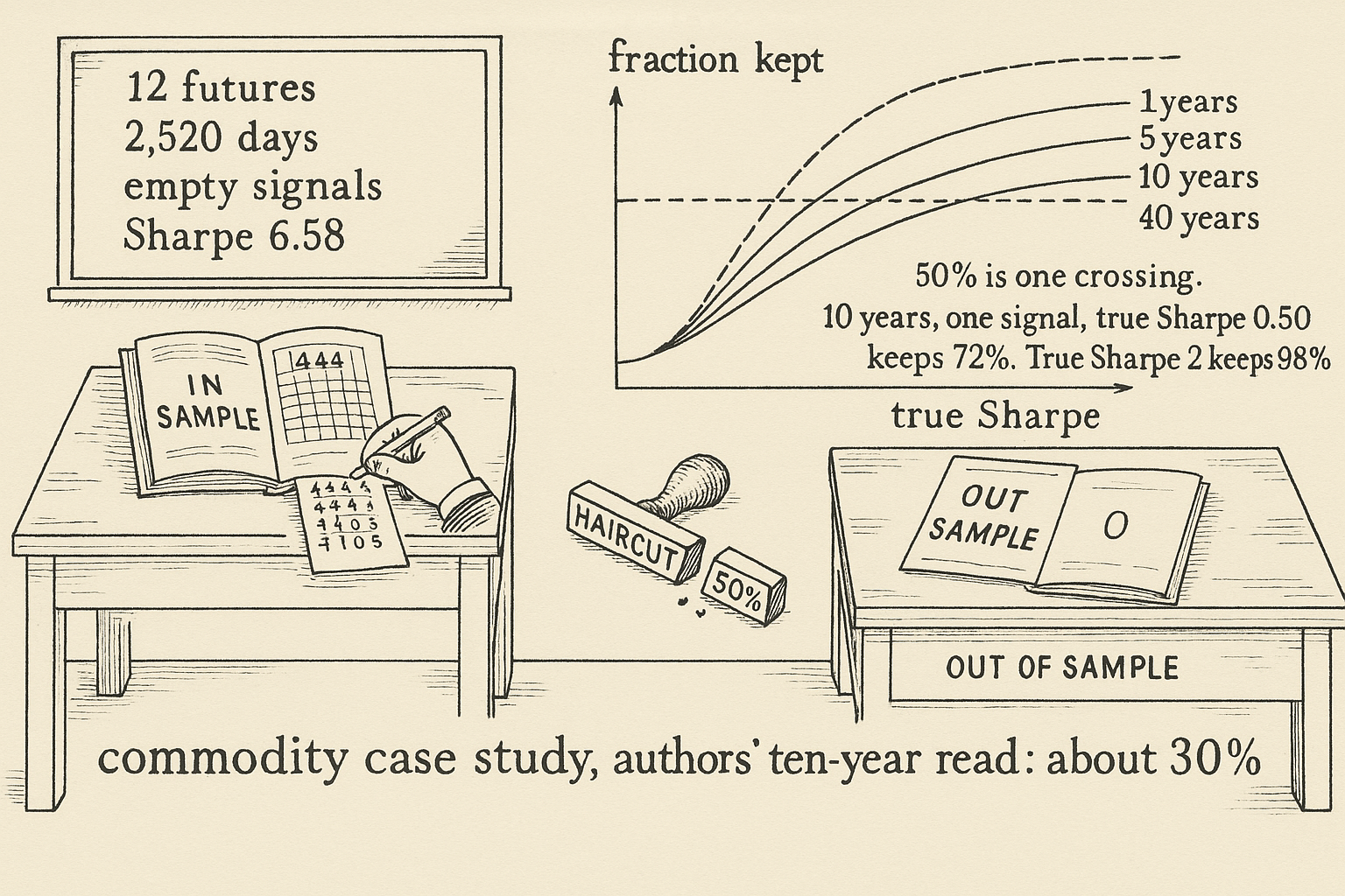
Sharpe ratio haircut: a 10-year commodity momentum fit keeps about 30% out of sample. The flat 50% rule is one cell, and often the wrong one.
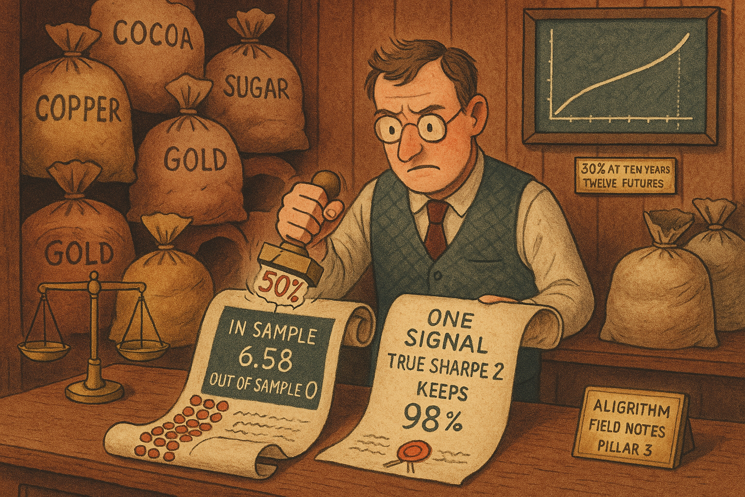
Twelve commodity futures, three momentum windows and an intercept, ten years of daily closes: 444 coefficients on 2,520 rows. Jacquier, Muhle-Karbe, and Mulligan compute the fraction of the in-sample Sharpe ratio this linear book is expected to keep on new data. Their commodity case study puts that fraction at 30 percent for a ten-year backtest. They attribute the rule of thumb that keeps 50 percent to Harvey and Liu. The fraction moves with the training length, the parameter count, and the true Sharpe. One future and one signal, true Sharpe 0.50: the formula keeps 20 percent after one year and 72 percent after ten. True Sharpe 2, ten years, still one signal: it keeps 98 percent. Twelve futures, 37 signals, a slope of zero, ten years: the in-sample Sharpe is 6.58 annualized and the fraction kept is zero.
What this actually is
You run twelve commodity futures, aluminium through sugar, and you fit a 5-day, a 1-year, and a 5-year momentum signal on each name, plus an intercept. That is 37 regressors and 444 coefficients. Ten years of closes is 2,520 rows. The backtest prints a Sharpe ratio, the mean profit-and-loss divided by its standard deviation, and you have to decide what fraction of it the same linear fit keeps on the next sample.
The method is a closed form for that fraction. It takes the signal count, the asset count, the number of training days, and the Sharpe the book would earn if the slopes were known. It returns an expected in-sample Sharpe and an expected out-of-sample Sharpe. Divide the second by the first.
Picture a student who sits the same exam twice. On the first sitting the answer key is on the desk, and every guess that matches the key is marked correct. On the second sitting the key is in the drawer. The drop equals those guesses. A short exam with a long question sheet drops harder. A long exam with one question the student knows keeps the first score.
At the desk you compute the fraction before you size the book. Keeping half of the 6.58 Sharpe that this 444-coefficient design prints when the true slope is zero would put on a book the formula sets to zero out of sample. Keeping half of one signal with a true Sharpe of 2, on ten years, throws away a book the formula says keeps 98 percent. The formula is too kind once you have discarded losing trials, and it charges no spread. Those bills sit in the old article "CSCV: A Direct Probability of Backtest Overfit" and the old article "The Backtest Integrity Checklist".
The in-sample mean carries an extra term
The question is why the backtest Sharpe sits above the live one even when you fit the regression once and never touch it again. The return model is linear. Tomorrow's return on each asset is a slope times today's signals, plus a residual.
$$ r_{t+1} = \beta s_t + \epsilon_{t+1} $$
Read it as a forecast. The vector r is next period's return on m assets, in return units per day. The vector s is today's signals, p of them, standardized in the formulas below to mean zero and unit variance. Beta is the m-by-p matrix of slopes, in return per unit of signal. Epsilon is the residual, mean zero, covariance sigma-epsilon. In the commodity fit, m is 12 and p is 37.
You estimate beta by ordinary least squares on the training window, then you trade the Markowitz book: weights equal the inverse residual covariance times beta times the current signal. The known-covariance assumption is deliberate. Estimating the covariance is a later section, and on twelve names the fraction stays put.
The fitted profit-and-loss splits into three pieces. The true piece is the book you would hold if beta were known. The misestimation piece multiplies the error in beta by the true expected return; its expectation is zero in the training window and out of it, because the residual mean is zero. The overfitting piece multiplies the error in beta by the residual itself. Inside the training window that residual is a row the regression already saw, and the expectation of that piece is not zero. Outside the window the residual is a fresh draw, and the expectation is zero. That is the entire mean gap.
$$ \mathbb{E}[\text{mean}_{\text{IS}}] = \operatorname{tr}(\Gamma) + \frac{p m}{T_1}, \qquad \mathbb{E}[\text{mean}_{\text{OOS}}] = \operatorname{tr}(\Gamma), \qquad \Gamma = \beta^{\top} \Sigma_{\epsilon}^{-1} \beta $$
Read it as two expected daily profit-and-loss figures, in the units of that Markowitz book, plus the gap between them. Gamma is a p-by-p matrix: beta-transpose times the inverse residual covariance times beta. Its trace is the daily profit-and-loss you would expect if the slopes were known. T1 is the number of training observations. The in-sample expectation adds p times m over T1. The out-of-sample expectation does not. This is their Proposition 3.1 for centred signals and Markowitz weights. The add-on is not a percent of net asset value. A constant rescaling of the weights scales the mean and the standard deviation together, so the Sharpe ratio, which is what you compare to a backtest, does not depend on that scaling.
Worked count for the commodity design: 12 times 37 is 444, and 444 divided by 2,520 is 0.1762. Every training day, the expected in-sample profit-and-loss sits 0.1762 above the expected out-of-sample profit-and-loss, in those units, at any true beta. Out of sample the add-on is zero. Add signals or add assets and the gap grows in a straight line. Lengthen the backtest and it shrinks as one over T1.
One asset and one signal
The question is what that gap does to the Sharpe ratio when there is only one slope to overfit. Set m = 1 and p = 1, scale the signal variance and the residual variance to 1, and leave the intercept out. The true per-day Sharpe, the one you would get with the slope known, collapses to a function of beta alone.
$$ \mathrm{SR} = \frac{\beta}{\sqrt{1 + 2\beta^{2}}} $$
Read it as a per-day Sharpe. Beta is the slope, in daily return per unit of signal, taken positive. Square root of 252 turns it into an annualized Sharpe under the model's own assumption that each day's profit-and-loss is independent of the last. The replication ratio below is a ratio of two Sharpes, so the square root of 252 cancels. It does not cancel on the horizontal axis of a chart drawn in annualized units, which is why the conversion is stated here.
Solve for the slope that delivers a true annualized Sharpe of 0.50. The square root of 252 is 15.8745, so the per-day Sharpe is 0.50 divided by 15.8745, which is 0.031497. Beta-squared equals 0.031497 squared, divided by 1 minus twice 0.031497 squared, which is 0.00099404. The true daily mean profit-and-loss in this scaling is that same 0.00099404. Add 1 divided by 2,520. The in-sample mean is 0.00139086. The ratio of the two means, 0.00099404 divided by 0.00139086, is 0.715.
The Sharpe ratio also has a variance, and the estimation error inflates it. Their simplified form of Proposition 3.1, for this one-asset case, is the pair below. Both are per-day Sharpes. The numerator is the expected profit-and-loss. The denominator is the square root of the expected variance. T1 is the training length in days.
$$ \mathrm{SR}_{\mathrm{EIS}} = \frac{\beta^{2} + 1/T_1}{\sqrt{2\beta^{4} + \left(1 + \dfrac{15}{T_1-2} - \dfrac{2}{T_1}\right)\beta^{2} + \dfrac{4}{T_1} - \dfrac{3}{T_1+2} - \dfrac{1}{T_1^{2}}}} $$$$ \mathrm{SR}_{\mathrm{EOOS}} = \frac{\beta^{2}}{\sqrt{2\beta^{4} + \left(1 + \dfrac{2}{T_1-2}\right)\beta^{2} + \dfrac{1}{T_1-2}}} $$
Read the first as the in-sample approximation and the second as the out-of-sample approximation. EIS is the ratio of the expected in-sample mean to the square root of the expected in-sample variance, and EOOS is the same construction on the new sample. They use this ratio-of-expectations because the expectation of the ratio has no closed form. In their checks the gap between the two stays within 2.5 percent of the Sharpe.
Plug in beta-squared of 0.00099404 and T1 of 2,520, which is the unrounded slope behind the 0.50 Sharpe. The in-sample variance is three terms: 0.000001976 from two times beta to the fourth, 0.000999168 from the slope term, and 0.000397612 from the estimation-noise constant. The sum is 0.001398756. Its square root is 0.037400. The in-sample mean, 0.00139086, divided by that square root, is a per-day Sharpe of 0.03719, and 0.03719 times 15.8745 is 0.590 annualized. The out-of-sample variance sums to 0.00139394. The per-day out-of-sample Sharpe is 0.02662, and the annualized figure is 0.423. Divide 0.4226 by 0.5904 and the fraction kept is 0.716. The ratio of the means alone was 0.715. In this cell the variance adjustment is a rounding error. Hold that thought for the twelve-asset book, where it is not.
$$ \text{Replication ratio} = \frac{\mathrm{SR}_{\mathrm{EOOS}}}{\mathrm{SR}_{\mathrm{EIS}}} $$
Read it as the fraction of the expected in-sample Sharpe that the expected out-of-sample Sharpe still covers. One means the backtest survives whole. Zero means the expected out-of-sample Sharpe is zero. The 50 percent rule is this ratio nailed to one half.
The same plug-in at other cells, all annualized by the square root of 252:
| Years | True Sharpe | In-sample | Out-of-sample | Fraction kept |
|---|---|---|---|---|
| 1 | 0 | 0.9903 | 0 | 0 |
| 1 | 0.50 | 1.1037 | 0.2231 | 0.202 |
| 1 | 0.983 | 1.3779 | 0.6890 | 0.500 |
| 10 | 0 | 0.3159 | 0 | 0 |
| 10 | 0.50 | 0.5904 | 0.4226 | 0.716 |
| 10 | 2.00 | 2.0198 | 1.9762 | 0.978 |
Check the 50 percent row before trusting the rest. Half of 1.3779 is 0.6890, and 0.6890 divided by 1.3779 is 0.500. That row is the folklore rule, and it is one cell: one asset, one signal, one year, a true Sharpe of 0.983. The crossings nearby sit at a true Sharpe of about 0.45 on five years, 0.32 on ten years, and 0.16 on forty years. A flat stamp of 50 percent is that curve's intersection with a horizontal line, read off at whatever sample length you happen to have.
On the one-year row with a true Sharpe of 0.50, the backtest is expected to print 1.10. Half of 1.10 is 0.55. The formula keeps 0.223. The stamp is more than twice too generous. On the ten-year row with a true Sharpe of 2, the backtest prints 2.02 and the formula keeps 1.98. Half of 2.02 is 1.01. The stamp throws away a Sharpe near 2. On a pure-noise signal the fraction kept is zero at every length, and a one-year sample still prints an in-sample Sharpe of 0.99. Half of 0.99 is a position. Zero is the out-of-sample number.
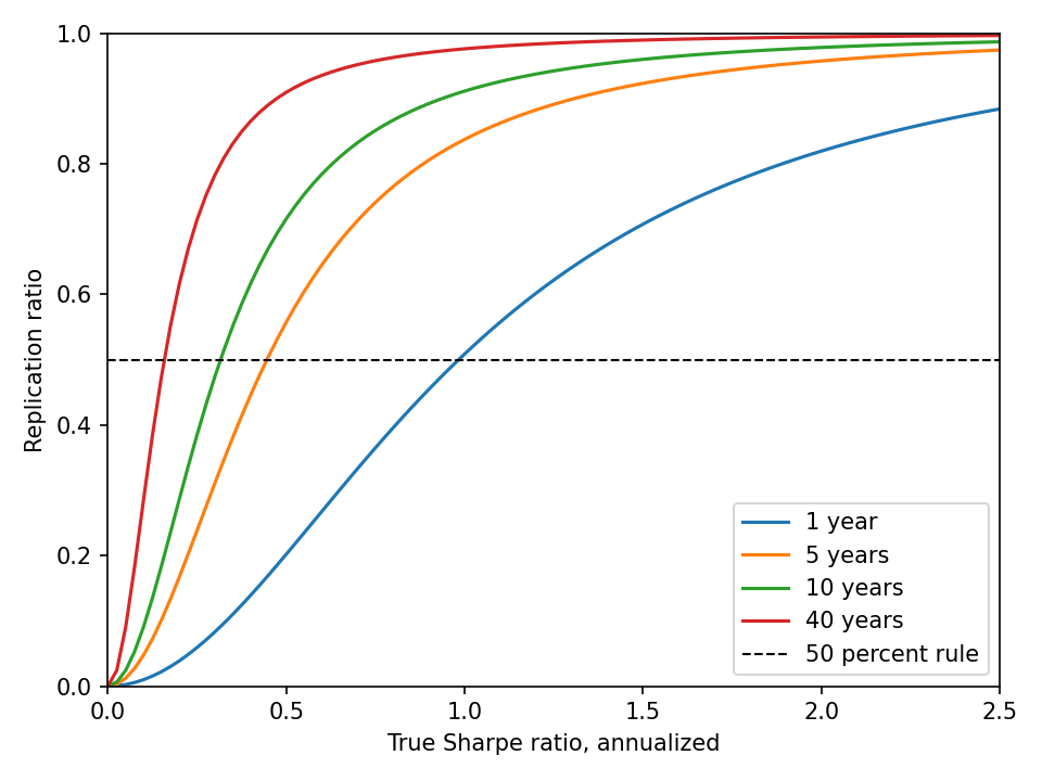
The curves are Proposition 3.1 in the one-asset case, not a fit to the commodity tape. A worthless signal sits at the origin. A strong signal on a long sample sits near one. The dashed line is the 50 percent rule, and each training length crosses it at a different true Sharpe.
Twelve assets, thirty-seven signals, a zero slope
The question is what this commodity parameter count prints when the signals carry nothing. Proposition 3.1 with a zero beta is exact on the variance side as well as the mean side: the leftover term they drop from the in-sample variance is a covariance between the inverse signal Gram matrix and a quadratic in beta, so a zero slope kills it.
Set m = 12, p = 37, T1 = 2,520, beta = 0, no intercept, known residual covariance, Markowitz weights. The in-sample mean is 444 divided by 2,520, which is 0.17619 per day. The in-sample variance reduces to two terms:
$$ \mathbb{E}[\mathrm{var}_{\mathrm{IS}}] = \frac{p m (2m + p + T_1 + 4)}{T_1 (T_1 + 2)} - \frac{2 m^{2} p^{2}}{T_1^{2} (T_1 + 2)} $$
Read it as a daily variance of the Markowitz profit-and-loss when the true slope is zero. The first term grows with the parameter count. The second subtracts a smaller piece that comes from the square of the mean. Evaluated here, the variance is 0.18057. That agrees with the long coefficient form in Proposition 3.1, the one with their c2 and c-tilde-2, digit for digit at this precision. The square root is 0.42493. Divide 0.17619 by 0.42493 and the per-day Sharpe is 0.4146. Times 15.8745, the annualized in-sample Sharpe is 6.58. The out-of-sample mean is zero, so the out-of-sample Sharpe is zero and the fraction kept is zero. The out-of-sample variance is 0.179, next to an in-sample variance of 0.181. The damage is the mean.
A 50 percent stamp on 6.58 leaves a Sharpe of 3.29 to trade. The formula leaves zero.
Two caveats sit on the 6.58. Proposition 3.1 drops the intercept. The commodity regression puts an intercept inside the 37 columns, so the variance terms shift once a column of ones is in the design, and 6.58 is the no-intercept null at this dimension. The mean gap does not shift: in the general expression the add-on is p over T1 times the trace of the weight matrix times sigma-epsilon, and for Markowitz weights that trace equals the asset count, so the add-on is still 0.1762 per day. And 6.58 is not a decomposition of the 8.2 they later report for a simulated book with a nonzero slope. Different beta, different number. The use of 6.58 is as a floor. A design of this size prints an annualized Sharpe above 6 on empty signals. An in-sample 8 has not cleared much.
The commodity case study prints two ten-year fractions
The question is what happened when they ran the design on commodity futures rather than on a zero slope. The universe is twelve names, May 1998 through December 2023: aluminium, copper, nickel, zinc, and lead on the LME; gasoil on ICE; WTI on NYMEX; gold and silver on COMEX; coffee, cocoa, and sugar on NYBOT. Signals are the 5-day, 1-year, and 5-year Sharpe ratio of each future, centred and scaled to unit variance, plus an asset-level intercept. They fit the simulator's beta by ridge with penalty 0.1, then draw 10,000 paths. Inside each path the traded book is ordinary least squares on that path. A path is 13 years at 252 days, 10 years in sample and 3 years out. Average correlation across signals is 20 percent, across residuals 28 percent. Average excess kurtosis of the residuals is 9. The diagonal of the fitted autoregressive matrix averages 0.88, a half-life of ln(2) over minus ln(0.88), which is 5.4 daily steps.
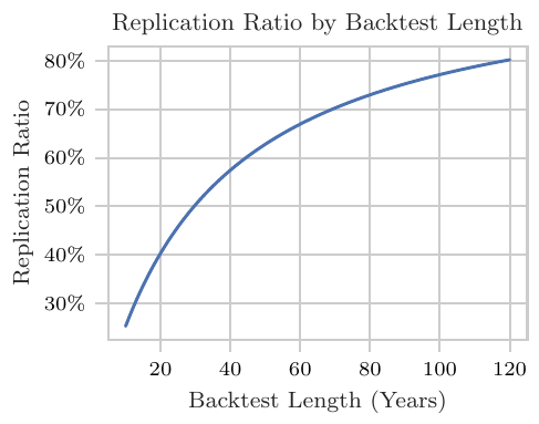
The authors read this curve as 30 percent at ten years, and it is still climbing through 80 percent out near 120 years. The parameter count is what pulls the fraction down there. A panel regression, one coefficient per momentum window shared across the twelve names, cuts the free parameters from 444 to 3.
The numbers they attach to that comparison do not all divide. In the simulation, where the data are drawn from the full model, they report an in-sample Sharpe of 8.2 and an out-of-sample Sharpe of 3.1 for the unrestricted book, and they call the replication ratio 38 percent. Those two Sharpes divide to 37.8 percent, so that pair checks. For the panel on the same simulated paths they report 0.9 in sample and 0.6 out of sample, and they call the ratio 70 percent. Divide 0.6 by 0.9 and you get 67 percent. On the real tape they report a panel ratio of 68 percent next to Sharpes of 0.7 and 0.5; 0.5 divided by 0.7 is 71 percent. They report an unrestricted ratio of 9 percent next to 3.6 and 0.3; 0.3 divided by 3.6 is 8.3 percent. An earlier sentence says a panel regression raises the replication ratio from 71 percent to 30 percent, which runs the wrong way, and which disagrees with both the 70-versus-38 simulation pair and the 68-versus-9 tape pair. The printed figures stay as printed. The ratios and the Sharpes do not reconcile, except the simulated unrestricted pair, and that one sentence has the direction backwards. The source may have swapped the 30 and the 71, or rounded the Sharpes past the point where the division survives. The paper also never shows the step that connects the 30 percent on the ten-year curve to the 38 percent in the simulation paragraph.
Read the pair that comes with Sharpes, and keep the conflict visible. In the simulation the fat model has the higher out-of-sample Sharpe, 3.1 against 0.6, because the paths were drawn from the fat model. The panel keeps a larger fraction of a smaller backtest. On the real tape the panel has the higher out-of-sample Sharpe, 0.5 against 0.3, and the unrestricted in-sample Sharpe of 3.6 falls to 0.3. The fraction kept and the level you earn are different questions. Keeping 70 percent of 0.9 leaves a smaller book than keeping 38 percent of 8.2, which is the simulation. On the tape the unrestricted 3.6 falls to 0.3. Prefer the panel when the tape says the extra coefficients are empty. Prefer it for the out-of-sample level, not for the prettier fraction.
The Gaussian, independent-signal simulation lands on the analytical values. They say the match is tight. Replacing the shocks with a t-distribution and the signals with an autoregression moves both Sharpes down and leaves the fraction close to the Gaussian number. Persistence has to get extreme before the independent-signal formula misleads: they put the gap against the independent case as small until the autoregressive coefficient exceeds 0.99. A coefficient of 0.9, which they describe as a half-life of 6.5 daily steps, is 6.6 steps if you compute ln(2) over minus ln(0.9). The fitted commodity diagonals, at 0.88, sit in the region where the formula still tracked.
Ten signals sit below the Kan, Wang, and Zheng curve
The question is how much of this is new relative to the constant-mean result. Kan, Wang, and Zheng have a closed form for the expected in-sample and out-of-sample Sharpe of a Markowitz book when the means and the covariance do not move, and the only thing you estimate is the mean vector. In this paper's language that is one signal per asset, and the signal never decays. Jacquier, Muhle-Karbe, and Mulligan add signals that die. At 2,520 observations in sample and the same count out of sample, with the true Sharpe fixed at 1.5, their one-signal curve lies on top of Kan, Wang, and Zheng as the asset count rises. Their ten-signal curve lies below it.
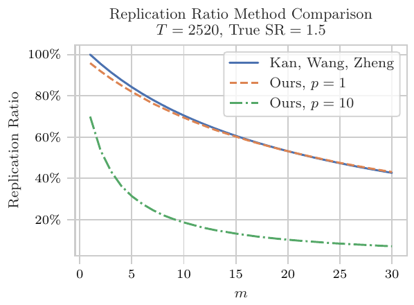
The true Sharpe is held fixed, so each extra signal is weaker. A new signal has to raise the true Sharpe by enough to pay for the drop in the fraction. Muller, in Quantitative Finance in 2001, said he would rather hold one strategy with a Sharpe ratio of 2 than stitch five uncorrelated Sharpe-1 strategies into a blend with a Sharpe ratio of 2.5. The one-signal row of the table above is that preference with a denominator: a true Sharpe of 2 on ten years keeps 98 percent. Five weak signals are a larger p, and the fraction falls.
The same moral shows up on the equity-premium side of the old article "Does Complexity Actually Help? The Virtue-of-Complexity Autopsy". There, a 15-predictor ridge beat a 12,000-feature timing model because the sample could not carry the coefficients. Here the bill is the Sharpe ratio itself, explicit in p, m, and T1. Kelly, Malamud, and Zhou are also the normalization this paper copies when it touches the Goyal, Welch, and Zafirov tape: returns divided by a trailing 12-month volatility, signals divided by an expanding volatility.
Where the formula stops
The question is which of your books this expression is allowed to tax. A few bounds are in the paper, and a few are outside it.
They drop a covariance term from the in-sample variance. In the commodity simulation that term was negative, and the simulated variance ran about 3 percent below the formula with the term set to zero. Across a wider draw of parameters the gap stays under 3 percent when the signal count over the training length is below 0.1, which is ten rows per signal. Thirty-seven signals on 2,520 days is 68 rows per signal, inside the bound. Thirty-seven signals on 252 days is 6.8 rows per signal, outside it. Do not quote the formula on a one-year fit of this design.
Estimating the residual covariance, instead of plugging in the true one, matches the known-covariance fraction at 12 assets and thousands of days. At 500 assets and a window shorter than the asset count, the sample covariance is singular and the out-of-sample Sharpe falls to about zero until the window exceeds the asset count. Their fix, once the asset count over the effective sample exceeds one, puts weight one over that ratio on the sample covariance and parks the rest on a scaled identity that preserves the trace. The slope error dominates the covariance error on the commodity book. On a 500-name book with a short window, the covariance error takes over.
The equity-premium check uses the Goyal, Welch, and Zafirov monthly predictors: 39 series with coverage somewhere in 1926 to 2024, random subsets of size 1 to 39, random windows of 10 to 70 years with both legs at least five years, five million draws. For each draw they pick a single scale k on the slope vector so that the analytical out-of-sample Sharpe matches the realized out-of-sample Sharpe. That match is by construction. The content of the test is whether the in-sample side, and therefore the fraction, lines up after you average across draws. They report that it does. More signals, lower fraction. Longer window, higher fraction. Higher implied true Sharpe, higher fraction. Read that figure as a check on the in-sample formula after the out-of-sample level has been pinned. Next year's Sharpe was an input to k.
Nothing here pays a spread, a borrow fee, or a missed fill. The old article "The Backtest Integrity Checklist" is the place those charges get applied, and a 30 percent statistical fraction is the input to that checklist, not the output. Nothing here prices the trials you threw away. The derivation is one regression, fit once. If you searched a stack of signal sets and kept the winner, this fraction is the damage from fitting that one winner, and the old article "CSCV: A Direct Probability of Backtest Overfit" is the damage from the search. Stack them. Do not substitute one for the other.
KEY POINTS
- The fraction of in-sample Sharpe a linear book keeps out of sample has a closed form. It falls as you add signals or assets, and it rises with the training length and with the true Sharpe. The commodity case study, as the authors read their curve, keeps 30 percent at ten years.
- The mean gap is p times m over T1. For 12 assets, 37 signals, and 2,520 days that add-on is 0.1762 per day in Markowitz units, at any true slope. Out of sample the add-on is zero.
- One asset, one signal, true annualized Sharpe 0.50: after one year the formula keeps 0.202 (in-sample 1.104, out-of-sample 0.223); after ten years it keeps 0.716 (in-sample 0.590, out-of-sample 0.423). A true Sharpe of 2 on ten years keeps 0.978. The 50 percent rule is the cell at one year and a true Sharpe of 0.983.
- With the intercept left out, 12 assets and 37 signals on 2,520 days and a zero slope print an in-sample Sharpe of 6.58 annualized and an out-of-sample Sharpe of 0. A 50 percent stamp would trade 3.29 of that. The commodity regression includes an intercept, so 6.58 is the no-intercept null, not a split of their simulated 8.2.
- In the simulation drawn from the full model they report unrestricted Sharpes of 8.2 in sample and 3.1 out of sample, ratio stated as 38 percent, and 3.1 divided by 8.2 is 37.8 percent. The panel pair 0.9 and 0.6 does not divide to the stated 70 percent (it divides to 67). On the real tape, 0.5/0.7 is 71 percent against a stated 68, and 0.3/3.6 is 8.3 percent against a stated 9. One sentence runs the panel effect backwards, from 71 percent to 30 percent. The ten-year curve's 30 percent and the simulation's 38 percent are also unreconciled in the paper.
- On the real tape the panel, 3 coefficients, has the higher out-of-sample Sharpe (0.5 against 0.3). In the simulation the fat model has the higher out-of-sample Sharpe (3.1 against 0.6), because the paths were drawn from it. Keep the fraction and the level as separate questions.
- The dropped variance term is about 3 percent in their commodity check, and under 3 percent when you have at least ten rows per signal. Covariance error is secondary at 12 names and dominant at 500 names on a window shorter than the cross-section. The equity-premium figure pins the out-of-sample Sharpe by construction and then checks the in-sample side. No spread is charged. Selection across many trials is a separate bill.
References
- Backtesting (Harvey, Liu, 2015)
- In-Sample and Out-of-Sample Sharpe Ratios of Multi-Factor Asset Pricing Models (Kan, Wang, Zheng, 2024)
- Dynamic Trading with Predictable Returns and Transaction Costs (Garleanu, Pedersen, 2013)
- A Comprehensive 2022 Look at the Empirical Performance of Equity Premium Prediction (Goyal, Welch, Zafirov, 2024)
- The Virtue of Complexity in Return Prediction (Kelly, Malamud, Zhou, 2024)
- Proprietary Trading: Truth and Fiction (Muller, 2001)
- In-Sample and Out-of-Sample Sharpe Ratios for Linear Predictive Models (Jacquier, Muhle-Karbe, Mulligan, 2025)
A note on AI. The ideas, research, analysis, and conclusions in this article are my own. I use AI tools to help with editing and wordsmithing, because English is not my first language, and I am not shy about that. AI-generated ideas and AI-assisted writing are not the same thing: the first is empty slop from a generic prompt, the second is a tool for communicating years of real research more clearly. Judge the work by its substance, not by whether software helped polish the prose.