10.19 Crypto Has Fundamentals: A Seven-Factor Model (Read Skeptically)

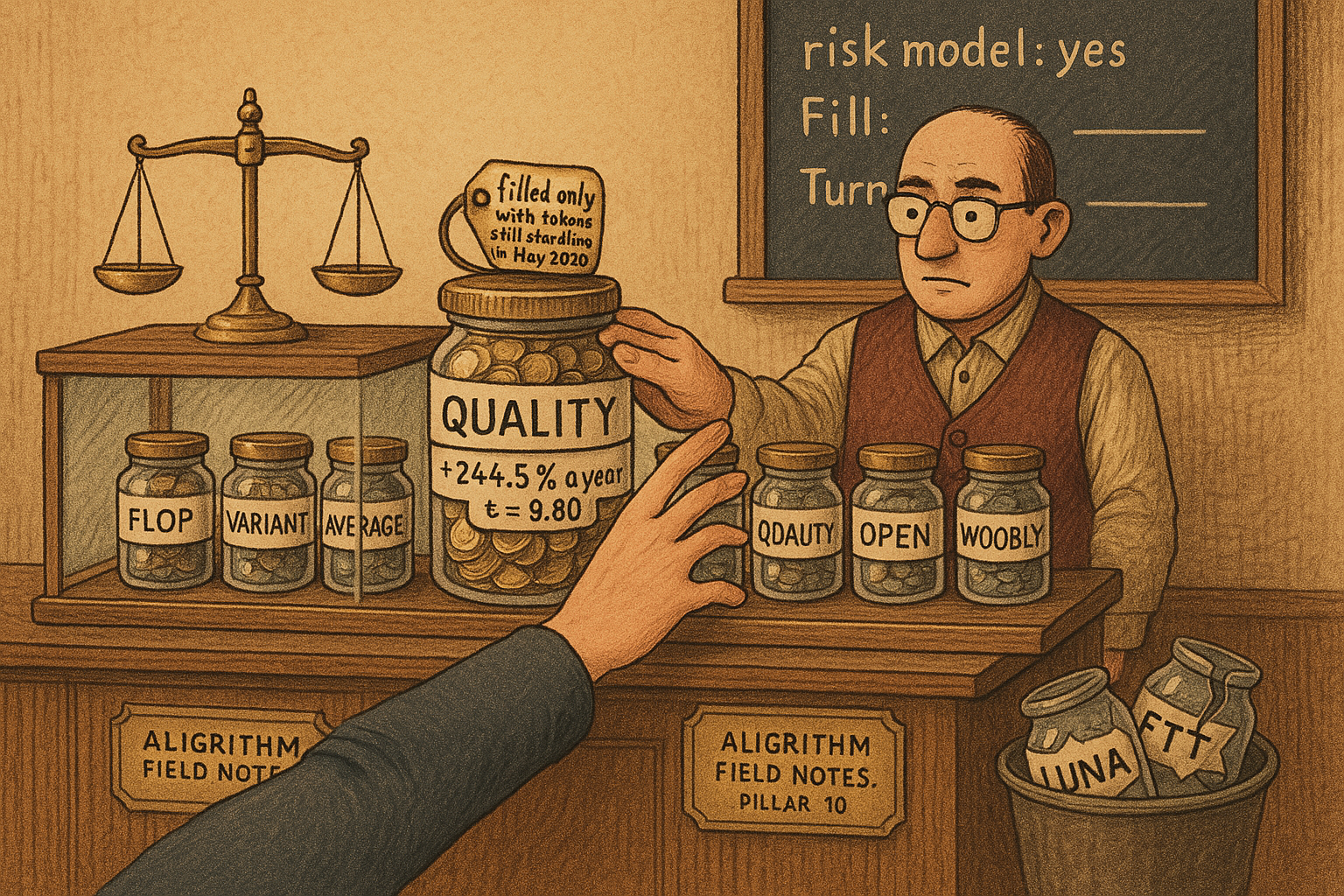
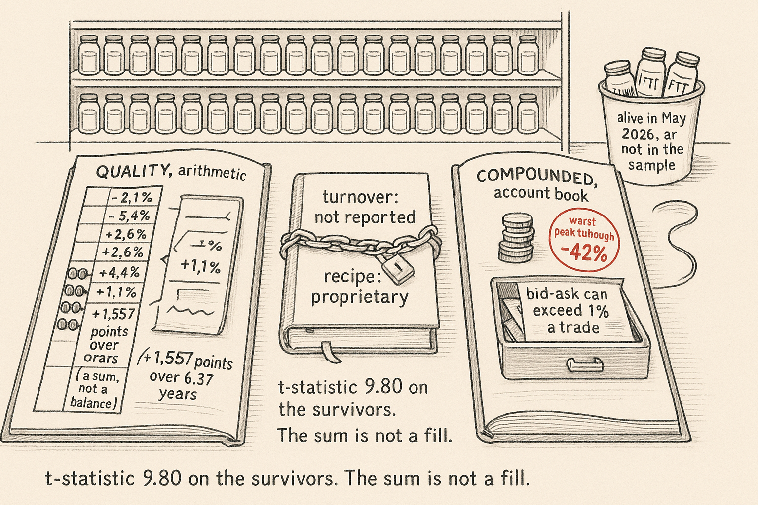
Babayev and Aliyev's on-chain quality factor posts a Newey-West t-statistic of 9.80 and a top-minus-bottom quintile return of 244.5% a year. The same paper builds its universe by keeping the 90 tokens still trading on 13 May 2026 and walking them backward, so LUNA and FTT never enter the short leg. A t-statistic of that size, on a sample that drops the tokens that died, describes the survivors. The authors say the spread is not a return you can implement. Read the model as a risk decomposition with that limit stapled to the front.

What this actually is

A book of tokens needs a split of yesterday's P&L. How much was the capitalization-weighted market, how much was a cluster of small names, how much was a bet that networks people use would beat networks they ignore. Without the split, a good month and an accidental factor tilt look identical, and the tilt cannot be hedged.

Q-7 is that split. Each day the authors score every token on seven characteristics, standardize the scores to a zero mean and a unit variance inside that day's cross-section, and regress the next day's return on the lagged scores. The average slope on a score is the premium attached to it.

Picture a landlord who ranks buildings by foot traffic, by rent relative to that traffic, and by how violent the street is, then checks whether the busy buildings paid more rent the next month. The rank is the factor. The extra rent is the premium. Throw out every building that collapsed before the study ends and the busy buildings look like a brilliant allocation, because the quiet ones that fell down are missing from the average.

If those slopes held up in a point-in-time universe, you would attribute a crypto book's P&L to the market, to sector, and to these style tilts, and you would hedge a quality exposure you did not mean to own. Treating 244.5% as a fill costs the bid-ask on names whose spreads the authors say can exceed 1% a trade, inside a quality score whose recipe they do not publish.

Seven scores, two of them unpublished

This section settles what each score computes, and which two you cannot rebuild.

Market (MKT) is the capitalization-weighted return of the universe, weights from yesterday's market cap, computed only when at least 10 tokens are present. Size (SMB) is the negative logarithm of that same lagged cap, so a small token receives a positive score. Reversal (REV) negates the 21-day cumulative return with a one-day skip, so a recent loser receives a positive score. Volatility (VOL) is the exponentially weighted standard deviation of the residual after a time-varying beta on the market, and the authors negate it, so a calm token receives the positive score. Funding (FND) is the perpetual-futures funding rate, negated and then residualized, so a token whose longs are paying shorts receives a negative score. A perpetual trading above spot has longs paying shorts every eight hours. The factor takes the other side of a high rate.

Value (VAL) and quality (QUA) are the unpublished pair. Value is a rank composite of five on-chain valuation ratios, each a market cap divided by some measure of network output, then residualized on size. Quality is a rank composite of four Coin Metrics activity series (unique participants, value transferred, transaction throughput, fees paid for block space), residualized on size and on value. Sakkas and Urquhart's earlier on-chain model was market plus a whale-concentration factor. This quality score is usage, and the formula is proprietary. The t-statistic of 9.80 sits on weights the paper does not print.

The residualizing is a cross-sectional regression of that day's scores. It is not a regression of the factor-return series on each other. Two factors can be uncorrelated as scores on a Tuesday and still move together as portfolios, because the names inside each quintile change and a market shock hits both books. Size and volatility still correlate at -0.56 as returns after the authors have stripped size out of the volatility score. Value and quality correlate at +0.35, which follows from both of them drawing on on-chain data for a similar subset of names. Funding's largest absolute return correlation is 0.17, against volatility.

The reversal window is the one place a desk can copy the construction without a vendor's black box. The paper says "21-day cumulative return" and does not write the price ratio. The reading below treats that phrase as the compounded change in price over the window. A sum of daily simple returns would differ on a token that moved this far.

$$ \mathrm{REV}_{i,t} = -\left(\frac{P_{i,t-2}}{P_{i,t-23}} - 1\right) $$

Read it as: for token i on day t, skip the most recent day, take the compounded return from the close 23 days ago to the close 2 days ago (21 trading days), and flip the sign. The price ratio is dimensionless. The score, before the cross-sectional z-score, is in return units. Worked example. A token that falls from 100 to 70 over that window has a compounded return of -0.30 and a raw reversal score of +0.30. A token that rises from 100 to 130 scores -0.30. After standardization, the loser is the name the long quintile wants.

The long-short itself is an equal-weighted quintile spread, rebuilt each day from lagged scores.

$$ R_{k,t} = \frac{1}{n_H}\sum_{i \in H} r_{i,t} - \frac{1}{n_L}\sum_{j \in L} r_{j,t} $$

Read it as: the factor return on day t is the average simple return of the top quintile H minus the average simple return of the bottom quintile L. Both averages are equal-weighted. The unit is a daily return. Worked quality. Table 6 prints the high-quality quintile at +187% a year and the low quintile at -58%. The difference is 245 percentage points. Table 4 prints 244.5%. The half point is rounding; Table 6 is in whole percentages. Quality's fourth quintile, at +190%, sits a hair above the fifth. Value is messier: the fourth quintile prints +192% and the fifth +157%, so the spread is carried by the extremes, and the middle of the sort bounces. The authors mark every row except volatility as "approximate" monotonicity. That label matches the table.

Coverage is uneven. Price-based scores cover the full 90 names. Quality covers 53 tokens and 62.1% of token-days, value 52 tokens and 60.6%, funding 89 tokens. A missing score enters the cross-sectional regression as a zero, a neutral loading. Quality's quintiles hold about 10 names. The sample runs from 2 January 2020 to 13 May 2026, 2,324 days, 170,006 token-days, 73 names a day on average, growing from 33 early in 2020 to 90 by late 2025. Sector dummies are membership flags. The counts are 38 Layer-1 names, 21 DeFi, 10 infrastructure, 9 Layer-2, 6 gaming, and 6 meme.

The annualized number is an arithmetic sum

This section settles the units on the 244.5%, because the cumulative chart is easy to misread as a wealth multiple.

$$ R^{\mathrm{ann}} = 365 \times \bar{r}, \qquad \sigma^{\mathrm{ann}} = \sqrt{365} \times s $$

Read it as: the annualized return is 365 times the mean daily simple return, and the annualized volatility is the square root of 365 times the standard deviation of the daily simple return. Both inputs are decimals per day. The outputs are decimals per year. This is an arithmetic convention. It is the one the paper states. Worked quality. 244.5% a year is 2.445 / 365 = 0.6699% a day. Volatility of 53.7% a year is 0.537 / 19.105 = 2.81% a day, where 19.105 is the square root of 365. Return divided by volatility, with a cash rate of zero, is 2.445 / 0.537 = 4.55. The paper does not publish a full-sample Sharpe ratio. The 4.55 is this ratio. The regime Sharpes in their sentiment table are the same ratio inside one bucket.

The cumulative chart sums the daily returns. The sample is 2,324 / 365 = 6.367 years long. Quality's 244.5% times 6.367 is +1,557 percentage points. Volatility's -234.4% times 6.367 is -1,492 percentage points. Market lands at +360, size at +159, reversal at +958, funding at +862, value at +1,175. The chart's quality line finishes above +1,500% and the volatility line finishes near -1,500%. The vertical scale of the figure is that multiplication.

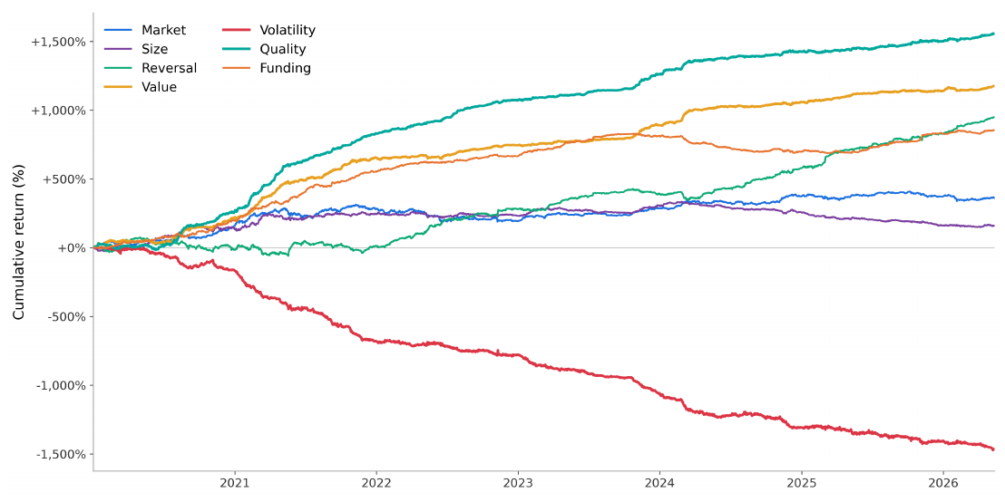
A constant 0.6699% a day, compounded for 2,324 days, finishes near 5.48 million times the starting stake. The natural log of 1.006699 is 0.006676, times 2,324 is 15.52, and e to that power is about 5.48 million. The chart does not show that path. The y-axis is the sum. Quality's worst peak-to-trough loss on the compounded wealth path is -42.2%, so that particular long-short did not go to zero inside the sample. The +1,557 label remains a sum of daily percentages. You cannot withdraw it.

The authors warn, above Table 4 and again in the limitations, that survivorship, transaction costs, and capacity cut these numbers hard. Bid-ask spreads on smaller tokens can exceed 1% a trade. They report no turnover, so there is no net figure to quote. A 1% round trip once a week removes 52 percentage points a year. A 1% round trip once a day removes 365 points, larger than the quality spread. Which frequency a live book would face is a turnover number they do not give. Treat 52 and 365 as a scale check.

The average token-day in the panel earned 0.15%. Under the same 365-day rule that is 54.8% a year, next to the capitalization-weighted market factor at 56.6%. Those are different series. One is the pooled token-day mean. The other is a cap-weighted portfolio. They happen to land close. On a given day the cross-section itself disperses by 4.74%, which the authors put at about 2.5 times the daily cross-sectional dispersion Fama and French reported for the S&P 500. A quintile sort has a wide field to work in. Costs are a separate test, and this paper does not run one.

Volatility got paid, and size dropped out

This section settles the sign of the volatility premium, including one sentence in the source that fights the tables.

Each day they regress token returns on the lagged z-scores. The premium is the average of those daily slopes. The t-statistic divides that average by a Newey-West standard error with five lags.

$$ r_{i,t} = a_t + \sum_k \lambda_{k,t}\, z_{i,k,t-1} + e_{i,t} $$

Read it as: token i's simple return on day t equals that day's intercept, plus a slope for each factor times the token's lagged z-score on that factor, plus a residual. The z-score is dimensionless. The slope lambda is a daily return per unit of z-score. The intercept is a daily return. Worked quality. The average slope is +0.003770. A token one cross-sectional standard deviation higher on quality earned 0.377% more the next day, in sample, with the other scores held fixed. Times 365, that is 137.6% a year per unit of z-score. Divide 0.003770 by the t-statistic 9.80 and the Newey-West standard error is 0.000385 per day. Volatility's average slope is -0.004572, t-statistic -9.19, which is -166.9% a year per unit of z-score. The negative sign is the construction. Low residual volatility received the positive score, high residual volatility earned the subsequent return, and the slope on the positive score came out negative. Baker, Bradley, and Wurgler documented the opposite pattern in equities, where the calm stocks earned the premium.

For volatility the autocorrelation adjustment raised the absolute t-statistic, from 7.46 with ordinary standard errors to 9.19 with five Newey-West lags. For quality it trimmed the t-statistic from 10.44 to 9.80. Five lags is their choice.

Divide the quintile spread by the annualized slope and the implied gap between the high and low quintiles is 1.78 z-scores for quality (2.445 / 1.376) and 1.40 z-scores for volatility (2.344 / 1.669). In a standard normal, the average of the top fifth sits 1.40 standard deviations above zero and the bottom fifth 1.40 below, a gap of 2.80. The paper never reports the average z-score inside each quintile. The slope is a partial coefficient on the in-sample window. The quintile spread is a raw sort on the full sample. The two printed numbers stand. Neither one gets edited to force a match.

Table 6's volatility row runs +223, +56, +42, +1, -12 from the column marked Q1 (Low) to the column marked Q5 (High). Q5 minus Q1 is -235 percentage points, against -234.4% in Table 4. The high score earned -12%. The low score earned +223%. Section 3.5 defines the high score as low residual volatility, because the signal is negated before the sort. Under that definition the calm tokens earned -12% and the jumpy tokens earned +223%, the same sign as the t-statistic of -9.19 and the same sign as the factor return of -234.4%. The sentence in section 4.3 says the +223% belongs to the lowest-volatility quintile and the -12% to the highest. That sentence conflicts with Table 4, with Table 6's column labels, with the signal definition, and with the t-statistic. The sentence stays as printed. The consistent set is the tables and the t-statistic. The source may have swapped "lowest" and "highest" in that one line.

Size's average slope is +0.000306, a t-statistic of 1.36, once volatility has been residualized on size. Annualized, that slope is 11.2% a year per unit of z-score. The size premium in earlier crypto work was this volatility premium. The authors keep size in the model as a control for value, quality, and funding, and because dropping it still costs 1.4 points of out-of-sample per-token R-squared.

The old article "What a Factor Actually Is: α + βλ, and Why the Market Is Factor #1" writes expected excess return as alpha plus beta-transpose lambda. The Fama-MacBeth slope is this paper's estimate of lambda. Quality's lambda is 0.377% a day per unit of z-score. The market, factor number one in that old article, still dominates the fit.

The 63% is mostly the market

This section settles what "63% out of sample" and "an in-sample/out-of-sample gap of -0.001" refer to. They are different regressions.

The split is June 2024. In sample: 1,626 days. Out of sample: 698 days. The two sum to 2,324, a 70/30 cut. The in-sample window holds the 2020-2021 rise, the 2022 break, and the recovery through mid-2024.

The cross-sectional R-squared is the average, across days, of the fit from that day's returns on that day's lagged scores. Style scores alone: 0.231 in sample, 0.274 out of sample. Style plus six sector dummies: 0.334 in sample, 0.335 out of sample. In-sample minus out-of-sample is -0.001. The raw cross-sectional fit did not fall after the split.

The adjusted row is the degrees-of-freedom haircut. With a raw R-squared of 0.334, 66 tokens, and 12 regressors (six style scores and six sector dummies), the adjusted figure is 1 minus 0.666 times 65/53, which equals 0.183. The paper prints 0.178. The 0.005 difference is what you get when the token count is not 66 on every day and the reported number is an average of daily adjusted R-squared values. The printed 0.178 stands. The same plug-in on the style-only row, raw R-squared 0.231 and six regressors, gives 0.153, which matches their adjusted in-sample figure to the digit they print. Out of sample, 90 tokens and 12 regressors turn a raw 0.335 into a plug-in adjusted value of 0.231, against their 0.234. The in-sample cross-sectional fit that survives the haircut is about 18%, on a cross-section of 66 names.

The 63% is a time-series regression, one per token. Regress the token's daily returns on the factor-return series, average the R-squared across tokens. Style plus sectors: 0.533 in sample, 0.632 out of sample. On this metric the fit rose after June 2024. The phrase "zero overfitting" in the paper is the cross-sectional gap of -0.001. The per-token R-squared moved from 0.533 to 0.632. Both numbers are in the paper. They answer different questions, and the second one went up.

A random equal-weighted portfolio of 30 tokens has an out-of-sample R-squared of 0.848, against 0.851 in sample. At 5 tokens the out-of-sample figure is already 0.760, at 10 tokens 0.803, at 20 tokens 0.835. Diversification removes the idiosyncratic noise, and the factor returns explain the common part. That is the attribution use the authors defend at the end.

Drop one factor and record the fall in the 0.632. The market costs 0.234 of R-squared, which is 0.234 / 0.632 = 37.0% of the fit, the share they print. Volatility costs 0.029. Size costs 0.014. Quality costs 0.004. They call quality's share 0.7% of the total; 0.004 / 0.632 = 0.63%, so the 0.7% is the rounded label. The factor with the t-statistic of 9.80 moves the average token's explained variance by 0.4 points, because the score exists for 53 of 90 names. A slope can be pinned down on the names you observe and still be a small piece of a 90-token book.

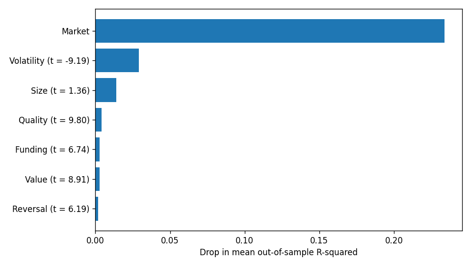
The old article "The Factor Zoo and the Multiple-Testing Reckoning" puts a practical hurdle near a t-statistic of 3 once a literature has tried hundreds of signals. A t-statistic of 9.80 clears that hurdle. The failure mode is the economic prior in that same old article. A premium this large has to show up as comovement, or it behaves like a near-arbitrage that costs and a point-in-time universe will take apart. Quality's full-sample return over volatility is 4.55. Its leave-one-out contribution is 0.4 points of R-squared. The return is large. The covariance footprint is small.

Losers won, except in greed

This section settles the sign fight with the earlier crypto factor model, and the sentiment split.

Liu, Tsyvinski, and Wu found that market, size, and momentum span the crypto cross-section, and that momentum subsumed the other price characteristics they tried. This sample, 90 tokens through May 2026, with data the authors say runs four years past that paper, finds the opposite sign at a 21-day horizon. The reversal t-statistic is 6.19. The quintile spread is 150.5% in the main factor table and 151.3% in the lookback table, with volatility 70.7% against 71.0% and the same -82% max drawdown. The paper presents both rows as the 21-day specification. The 0.8 point gap in the annualized return is unexplained. Both figures stay as printed.

Shorter windows print larger arithmetic returns and a compounded max drawdown of -100%. Seven days: +266.1% annualized, volatility 81.5%, max drawdown -100%. Fourteen days: +200.1%, drawdown -100%. Forty-two and 63 days also print a -100% max drawdown, at +109.5% and +115.7% annualized. The 21-day row is the specification whose drawdown is -82%. A -100% max drawdown means the compounded long-short touched zero, while the 365-day annualization of the mean still printed a triple-digit gain. The fast reversal book went bust inside the backtest on the compounded path.

A sector-neutral variant, standardizing the 21-day return inside each sector before ranking, prints +202% against the raw +151% the authors quote. The reversal lives inside the sector.

The old article "Percentile-Rank Momentum With Hysteresis: Low-Churn Signals" builds a continuation signal on Bitcoin and Ethereum and spends its engineering on a band that stops the position flipping every time the sign changes. A desk running that continuation book and this paper's 21-day reversal book stands on opposite sides of a recent loser. The horizon where this paper's arithmetic return is largest already shows a -100% drawdown.

Sentiment uses the Alternative.me Fear and Greed index, smoothed over 30 days, cut at 35 and at 65. Fear, below 35: 746 days. Neutral, 35 to 65: 947 days. Greed, above 65: 613 days. The three sum to 2,306, eighteen days short of the 2,324-day return sample. The authors call the shares 32%, 41%, and 27%. Dividing by 2,306 gives 32.4%, 41.1%, and 26.6%.

Reversal in fear: +234.6%, Sharpe ratio 3.75, so volatility inside that bucket is 234.6 / 3.75 = 62.6%. Reversal in greed: -5.1%, Sharpe ratio -0.07. Value runs the other way: +93.9% in fear, +365.2% in greed at a Sharpe ratio of 6.10, implied volatility 365.2 / 6.10 = 59.9%. Quality stays positive in all three buckets: +183.5% in fear (Sharpe ratio 4.16), +177.6% in neutral (Sharpe ratio 3.50), +424.4% in greed (Sharpe ratio 6.37). The greed-regime quality Sharpe ratio of 6.37 implies a volatility of 424.4 / 6.37 = 66.6%, against 53.7% on the full sample. Funding stays between +128.0% and +140.6%. Volatility is negative in every regime and worst in greed, at -452.1%, Sharpe ratio -4.82.

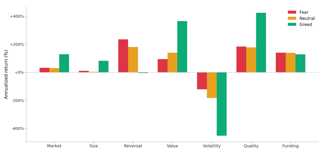
A Sharpe ratio of 6.37 on a 613-day greed subsample, inside a survivor universe, with no costs, is the object the economic prior was written to catch. The cross-sectional R-squared stays at 0.331, 0.344, and 0.323 across the three buckets. The fit is stable. The premia move around. Conditioning a tilt on this index is an in-sample cut, and the authors say it wants a further test.

In this sample the sentiment index ran with the market. Its correlation with the forward 63-day market return is +0.16, t-statistic 7.52. Square 0.16 and you get 0.0256, the predictive R-squared they describe as under 3%.

Keep the attribution, leave the spread

Use the decomposition. On a 30-token equal-weighted book the factor returns explain 85% of return variance out of sample (0.848, which rounds to the 85% in the abstract), and the market accounts for 23.4 points of the 63.2-point per-token fit. Attribute the month to the cap-weighted market, to sector, and to the style tilts the holdings happen to carry. Hedge the tilt you did not want.

Leave the quintile spreads on the page. Quality at 244.5%, value at 184.5%, reversal at 150.5%, and funding at 135.4% are arithmetic long-short means on a universe defined as tokens still alive on 13 May 2026. The authors name the bias and the mechanism: the tokens that survived are the ones with high network use and enough capitalization, which is what the quality and value scores select. Both formulas are unpublished. Coverage is 53 and 52 names. Turnover is unpublished. Spreads on the small names can exceed 1% a trade. Funding, the score closest to orthogonal in the return correlations, is still a 135.4% gross spread with a -78.3% max drawdown and no cost model.

Q-7 is a sketch of the attribution split. The 244.5% stays in the table.

KEY POINTS

• Q-7 scores tokens on market, size, 21-day reversal, on-chain value, residual volatility, on-chain quality, and perpetual funding. Value and quality are proprietary rank composites. You cannot rebuild the t-statistic of 9.80 from the paper.
• Quality's top-minus-bottom quintile earns 244.5% a year arithmetic (Table 6's quintiles differ by 245 points). That annualization is 365 times the mean daily return, 0.6699% a day. Summed over 2,324 days it is +1,557 points, which is the vertical scale of the cumulative chart. Compounding that same daily rate over 2,324 days produces a multiple near 5.48 million. The chart is the sum.
• The Fama-MacBeth slope on quality is +0.377% a day per unit of z-score (137.6% a year), Newey-West t-statistic 9.80. Volatility's slope is -0.457% a day, t-statistic -9.19, because the positive score is low residual volatility and the jumpy tokens earned the return. One sentence in section 4.3 swaps those quintile names; the tables and the t-statistic agree with each other.
• Size's t-statistic falls to 1.36 once volatility is residualized on size. The apparent size premium was a volatility premium. Size stays in the model as a control.
• Per-token out-of-sample R-squared is 0.632 with sectors, and a 30-token book reaches 0.848. The market's leave-one-out share of the 0.632 is 0.234. Quality's is 0.004. The cross-sectional in-sample/out-of-sample gap of -0.001 is a different regression from the per-token R-squared, which rose from 0.533 to 0.632.
• This sample finds 21-day reversal (t-statistic 6.19, about +151% a year), where Liu, Tsyvinski, and Wu found continuation. The 7-day version prints +266% and a -100% max drawdown. Reversal earns +235% in fear and -5% in greed. Quality's greed-regime Sharpe ratio is 6.37.
• The universe is tokens alive in May 2026, projected backward. The authors say this inflates every factor return, and that quality and value select the characteristics survivors have. Use the model to attribute a book's P&L. Leave the quintile spreads in the table. Turnover is unreported, and smaller-token spreads can exceed 1% a trade.

References

• Liu, Tsyvinski, and Wu (2022). Common Risk Factors in Cryptocurrency
• Sakkas and Urquhart (2024). Blockchain Factors
• Babayev and Aliyev (2026). Crypto Has Fundamentals: A Seven-Factor Model for Digital Asset Returns

A note on AI. The ideas, research, analysis, and conclusions in this article are my own. I use AI tools to help with editing and wordsmithing, because English is not my first language, and I am not shy about that. AI-generated ideas and AI-assisted writing are not the same thing: the first is empty slop from a generic prompt, the second is a tool for communicating years of real research more clearly. Judge the work by its substance, not by whether software helped polish the prose.