10.1 What a Factor Actually Is: α + βλ, and Why the Market Is Factor #1
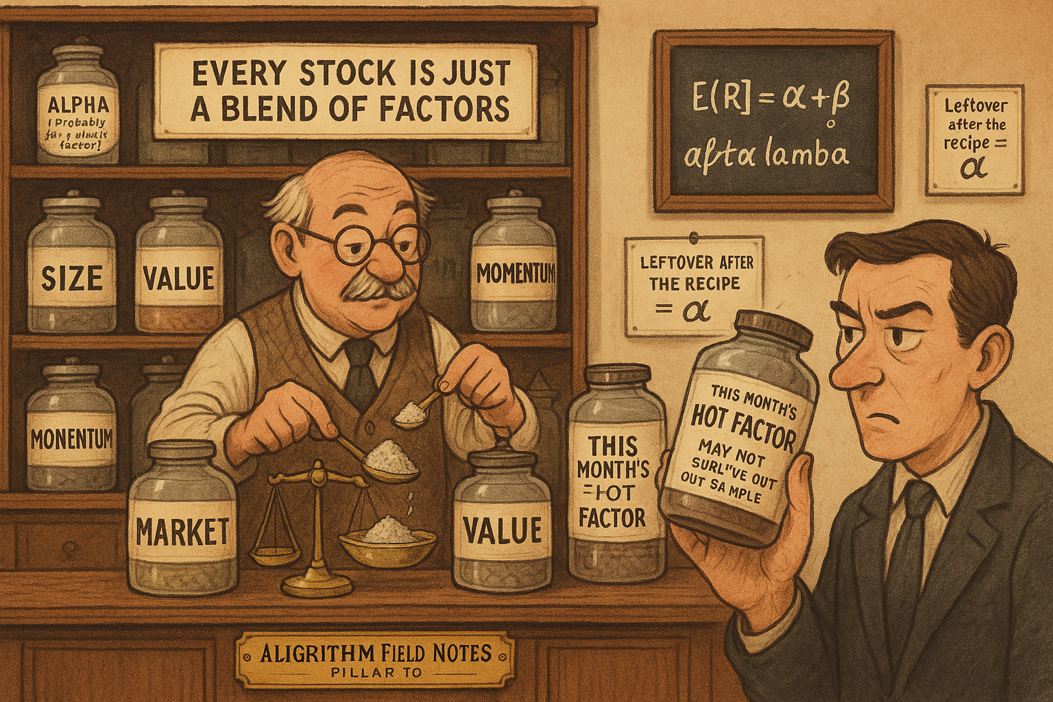
Factor investing runs on one equation: expected return equals alpha plus beta times lambda. Beta is exposure, lambda is the premium, alpha is the leftover. The market is factor #1, and CAPM fails on its own.
Pull fourteen years of returns for Alphabet and Citigroup. One compounds to roughly ten times your money, the other crawls sideways near two. The reflex is to explain each path on its own: Google had better products, Citi carried a bad balance sheet through the crisis. That reflex is the wrong axis. The question underneath factor investing is not "where does this one stock go next," it is "why do average returns differ across the whole cross-section of stocks at the same time." Answer that and you stop trading stories about single names and start trading the thing that actually separates the winners from the losers.
The old article "What Is a Factor, Really" gave the practitioner's version of the answer: a factor is an alpha that explains so much return variance you keep re-finding it, so you subtract it before hunting for new edge. This article gives the equation that both the academics and the fund managers are arguing over when they say the word "factor," and shows they are staring at the same three symbols from opposite ends.
The one equation everything hangs on
Every factor model, from a 1960s single-market story to a 2020s neural net, is a claim about one line:
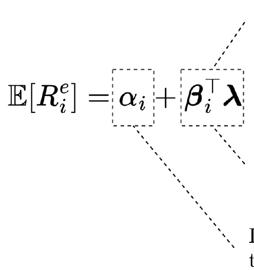
$$ \mathbb{E}[R_i^e] = \alpha_i + \beta_i^\top \lambda $$
Read it left to right. The term on the left, expected excess R, is the asset's average return above the risk-free rate. Lambda is a vector of factor risk premiums, the extra return the market pays for holding each factor. Beta is that asset's vector of exposures, how much of each factor it carries. The dot product beta-transpose lambda is the return the model says the asset earns for its exposures. Whatever the equation cannot account for lands in alpha, the pricing error.
Work a number through it. Say a stock loads 1.2 on the market, 0.4 on value, and −0.3 on momentum, and the annual premiums are 6% for the market, 3% for value, and 4% for momentum. The model return is 1.2 times 6, plus 0.4 times 3, minus 0.3 times 4, which is 7.2 plus 1.2 minus 1.2, so 7.2% a year. If the stock actually averaged 9%, the leftover 1.8% is its alpha. If it averaged 7.2%, its alpha is zero and the factors explained everything.
That leftover is the whole game. A significant nonzero alpha means either your model is missing a factor, or the asset is genuinely mispriced, or you got fooled by a small sample. The equation itself does not tell you which. It just quarantines the part you cannot explain and dares you to explain it.
The market is factor number one, and it fails on its own
The first factor anyone wrote down was the market. The Capital Asset Pricing Model says an asset's expected excess return is its market beta times the market's excess return, and nothing else:
$$ \mathbb{E}[R_i] - R_f = \beta_i \big( \mathbb{E}[R_M] - R_f \big) $$
One factor, one premium. High-beta stocks should earn more, low-beta stocks less, in a straight line through the origin. The market is factor number one for the same reason the old article "What Is a Factor, Really" strips market beta before anything else: it explains more return variance than any characteristic you will ever measure, so it contaminates every other signal you test. Remove it first because it is the biggest liar in the room about whether you found something new.
The trouble is that the line does not hold. Sort real stocks by beta and average their returns, and the relationship goes flat, then bends down at the high-beta end.
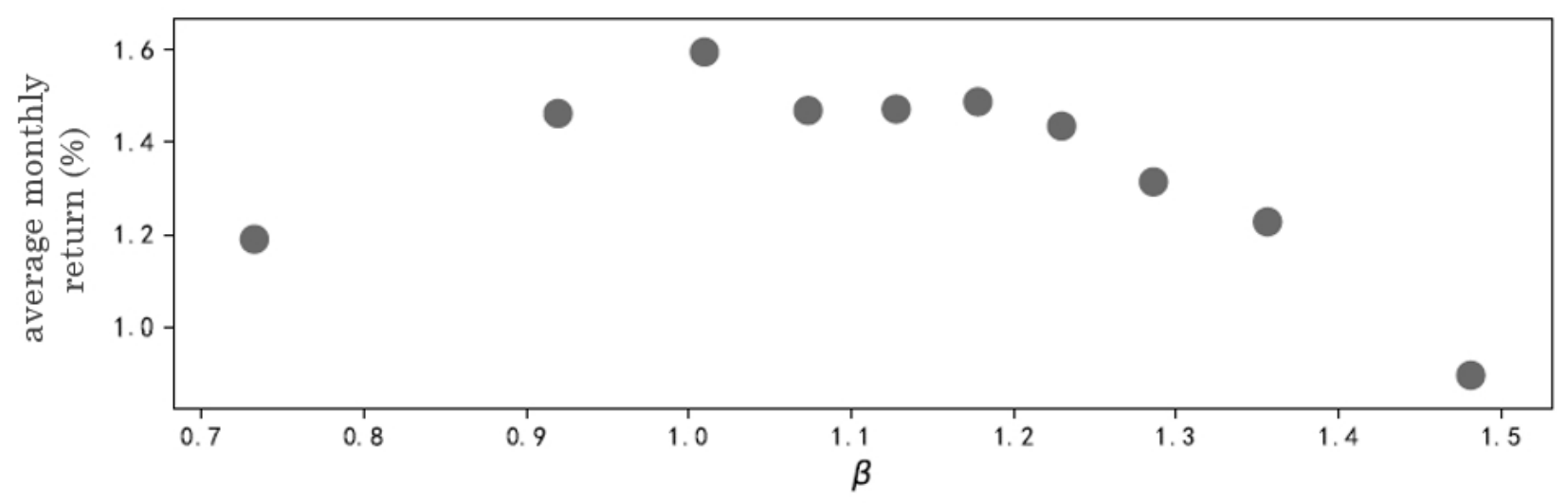
Returns climb a little from a beta of 0.7 to about 1.0, then stall, then slide as beta keeps rising. The stocks with the most market risk did not earn the most return. That single scatter killed CAPM as a complete story and forced the field to admit that expected returns depend on more than one exposure. Ross packaged the fix in Arbitrage Pricing Theory: keep the linear form, add more factors, and the market becomes the first term in a longer sum rather than the only term. Size showed up (small beats large), then value (cheap beats expensive), and the single-factor world was over.
Two conditions, or it is not a factor
A characteristic that predicts returns is not automatically a factor. The paper's definition sets a bar with two conditions, and both have to clear.
First, the factor has to drive the common co-movement of asset returns, which means it has to show up in the covariance matrix. Second, it has to be priced, meaning holding exposure to it earns you a premium over time. Miss either one and you have a curiosity, not a factor.
The cleanest intuition is that factors are to assets as nutrients are to food.

A meal is a bundle of nutrients; a stock is a bundle of factor exposures. You do not eat "protein" directly, you eat chicken that carries protein, and you do not buy "value" directly, you buy a cheap stock that carries value loading. The analogy also flags the skeptic's job. Plenty of characteristics correlate with returns in one sample and vanish in the next, which is the equivalent of a fad ingredient that turns out to do nothing. Whether a proposed factor survives the "is it priced out of sample" test is the entire content of the factor-zoo problem, and most of the roughly three-hundred published factors do not survive it. That reckoning gets its own article; here the point is narrower. Both conditions are load-bearing, and the second one is where the graveyard fills up.
Alpha is a test of the market, and a trap for the researcher
Once you accept the equation, alpha stops being a bragging number and becomes a diagnostic. When a long-short portfolio built on some sorting variable shows a significant nonzero alpha against your factor model, that portfolio is an anomaly, and the variable is an anomaly variable. Academics care about this because a real anomaly challenges market efficiency: if the market priced everything correctly, no characteristic should leave a systematic alpha behind.
Fama named the catch. You can never test market efficiency by itself, because you always test it jointly with whatever pricing model you assumed. This is the joint hypothesis problem. A nonzero alpha means the market is inefficient, or your model is wrong, and the test cannot separate the two. The side effect poisoned decades of research. If a nonzero alpha just means "add a factor," the lazy move is to keep adding factors until the alpha disappears in-sample. That is curve-fitting with a respectable vocabulary, and it is the cross-sectional cousin of the overfitting the robustness articles keep warning about. The academy's habit of chasing the model that minimizes pricing errors in-sample manufactured a large share of the factor zoo it now cannot replicate.
The industry reads the same alpha differently. A fund manager does not want alpha to test a philosophy of markets, the manager wants alpha to survive transaction costs and land in the P&L. Same symbol, opposite motive. One camp uses alpha to grade a theory, the other uses it to grade a trade.
The same equation, read from both ends
Split the equation into its two moving parts and the academia-versus-industry split becomes obvious. Nobody is disagreeing about the math. They are pointing at different terms.
| Term | Academia asks | Industry asks |
|---|---|---|
| beta-transpose lambda | Which is the "best" factor model? What are the true premiums? | Which factors carry a positive premium I can allocate to? |
| alpha | Is the market efficient? Is model A better than model B? | Can I earn this after costs, and how do I attribute my fund's return? |
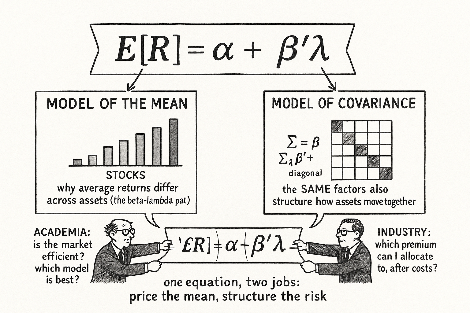
The beta-transpose lambda term is the model of the mean, the part that explains why average returns differ across assets. Academics fight over the correct list of factors and the econometrics for estimating premiums, using alpha to compare models where fewer surviving anomalies means a better model. Fund managers take the factors as given, look for the ones with durable positive premiums, and load up exposure under a diversification budget, which is exactly what the smart-beta ETF industry sells. Ranking a whole universe on a characteristic and holding the top against the bottom is the cross-sectional engine behind the old articles "Ranking Beats Forecasting for Many Trading Problems" and "Order Book Imbalance: The First Microstructure Feature to Test," where imbalance is treated as the first thing to rank on at the tick level.
Model of the mean, model of covariance
The equation you have been reading is the cross-sectional view, one expected return per asset. Run the same relationship through time and it becomes a regression of each asset's realized excess return on the factor realizations:
$$ R_{it}^e = \alpha_i + \beta_i^\top \lambda_t + \varepsilon_{it} \qquad\Longrightarrow\qquad \Sigma = \beta \, \Sigma_\lambda \, \beta^\top + \Sigma_\varepsilon $$
The left piece is the time-series version: this month's return equals the constant alpha, plus the exposures times this month's factor returns, plus an idiosyncratic shock. Take the covariance of both sides, use the fact that factor returns and shocks are uncorrelated, and you get the right piece. The full covariance matrix of assets, Sigma, splits into a systematic part driven by the factors, beta times the factor covariance times beta-transpose, plus a diagonal matrix of stock-specific variances. This is the model of covariance, and it is the same factors doing double duty.
The payoff is practical, not decorative. Estimating a raw covariance matrix for N assets needs at least N periods of data, or the sample matrix is singular and useless. A five-factor model replaces the N-by-N estimation problem with a handful of factor covariances plus N diagonal terms, which is why risk models are built as factor models. The factors that explain the mean return are the same ones that structure the risk. That is not a coincidence the theory tolerates, it is the theory's central claim: if a characteristic prices the cross-section of returns, it should also organize how those returns move together, and if it does one without the other, it fails the definition.
Where this connects
The equation expected excess return equals alpha plus beta-transpose lambda is the spine of this whole pillar. Portfolio sorts estimate the lambda term by ranking and spreading. The GRS test asks whether the whole vector of alphas is jointly zero. Fama-MacBeth estimates the premiums in a second pass. The factor zoo is the fight over how many terms belong in the sum before you are just fitting noise. Every one of those is a move on this single line.
It also reaches back into the earlier pillars. Predicting the residual instead of the gross return, the thesis of the old article "Predict Residual Returns, Not Gross," is the same instinct as forecasting alpha after the factors are removed. Benchmarks, the subject of "Why Benchmarks Matter in Rule Evaluation," are just the beta-transpose lambda an honest test subtracts before crediting you with skill. Name the systematic part, remove it, and pay attention only to what survives. The equation is the bookkeeping that makes that discipline exact.
KEY POINTS
- Factor investing asks a cross-sectional question, why average returns differ across assets at the same time, not a time-series question about where one stock goes next.
- Everything hangs on one equation: expected excess return equals alpha plus beta-transpose lambda. Beta is exposure, lambda is the factor premium, and alpha is whatever the model cannot explain.
- The market is factor number one because it explains the most return variance, so you remove it first. CAPM says returns rise in a straight line with beta, but real data bends flat then downward, which is what forced multi-factor models.
- A factor has to clear two conditions: it must drive the common co-movement of returns (show up in the covariance matrix) and it must be priced. Most published factors fail the second test out of sample.
- Alpha is a diagnostic, not a trophy. A significant alpha means a missing factor, a real mispricing, or a small-sample fluke, and Fama's joint hypothesis problem says you cannot cleanly separate the first two. Minimizing alpha in-sample by piling on factors is curve-fitting with a respectable name.
- Academia and industry read the same equation from opposite ends: academics fight over the best model and use alpha to test efficiency, managers take the factors as given and allocate to durable premiums after costs.
- The cross-sectional equation has a time-series twin whose covariance splits as Sigma equals beta Sigma-lambda beta-transpose plus a diagonal. The factors that price the mean are the same ones that structure the risk, which is why risk models are factor models.
References
- The Arbitrage Theory of Capital Asset Pricing (Ross, 1976)
- Common Risk Factors in the Returns on Stocks and Bonds (Fama and French, 1993)
- A Five-Factor Asset Pricing Model (Fama and French, 2015)
- Digesting Anomalies: An Investment Approach (Hou, Xue, and Zhang, 2015)
- A Census of the Factor Zoo (Harvey and Liu, 2019)
- Shrinking the Cross-Section (Kozak, Nagel, and Santosh, 2020)
- A Test of the Efficiency of a Given Portfolio (Gibbons, Ross, and Shanken, 1989)
- Presidential Address: Discount Rates (Cochrane, 2011)
- Arbitrage Asymmetry and the Idiosyncratic Volatility Puzzle (Stambaugh, Yu, and Yuan, 2015)
A note on AI. The ideas, research, analysis, and conclusions in this article are my own. I use AI tools to help with editing and wordsmithing, because English is not my first language, and I am not shy about that. AI-generated ideas and AI-assisted writing are not the same thing: the first is empty slop from a generic prompt, the second is a tool for communicating years of real research more clearly. Judge the work by its substance, not by whether software helped polish the prose.