10. Cross-Sectional & Factor Investing July 8, 2026 11 min

10.2 Portfolio Sorts From Scratch: Deciles, Monotonicity, and the Long-Short Spread

You never see factor exposure. So you rank stocks on a proxy, go long the top decile and short the bottom, and test the spread. Deciles, a t-stat, and a monotonicity check, from scratch.

The old article "What a Factor Actually Is" ended on the equation expected excess return equals alpha plus beta-transpose lambda, and left a hole. Lambda is the factor premium, the number you actually get paid. But you never observe a stock's factor exposure, and you never observe lambda directly either. Both are hidden. So how does anyone put a number on the value premium or the size premium? They sort. Portfolio sorts are the workhorse that turns a characteristic you can measure into a factor return you can trade, and they are the first thing any factor claim has to survive. Get the sort wrong and every t-stat downstream is noise.

The trick is to stop pretending you can measure exposure. You can't read a stock's true loading on the value factor off a screen. What you can read is its book-to-market ratio, and the sort assumes only that book-to-market is correlated with the value loading. Not equal to it, not a linear function of it, just correlated in the right direction. That weak assumption is the whole method, and it is why sorting is more honest than regressing returns on a characteristic and pretending the coefficient is a premium.

Rank on a proxy, not a measurement

In a portfolio sort the variable you rank on is the sorting variable, and book-to-market is the classic one. The method uses that variable as a stand-in for exposure to the factor. High book-to-market means "probably high value loading," low book-to-market means "probably low value loading," and that is all it claims. No functional form, no assumption that a book-to-market of 2.0 means twice the loading of 1.0. The only requirement is that the ranking lines up with the exposure often enough.

This is the same instinct as the old article "Ranking Beats Forecasting for Many Trading Problems." You do not need to predict the magnitude of a stock's return to trade the cross-section, you only need to get the order roughly right, because expected returns are tiny next to their own standard error and any point forecast of them is mostly noise. Sorting throws the magnitude away on purpose and keeps the order. A monotone error in your proxy leaves the ranking intact, so the sort survives a badly calibrated signal in a way a return regression does not. The old article "Cross-Sectional Percentile Rank Within a Universe" ran the same play from the indicator side, ranking one market's normalized trend against its peers. A Fama-French decile sort is that idea industrialized across a few thousand stocks.

The three-step recipe

The mechanics are boring, which is the point. Boring means fewer places to cheat.

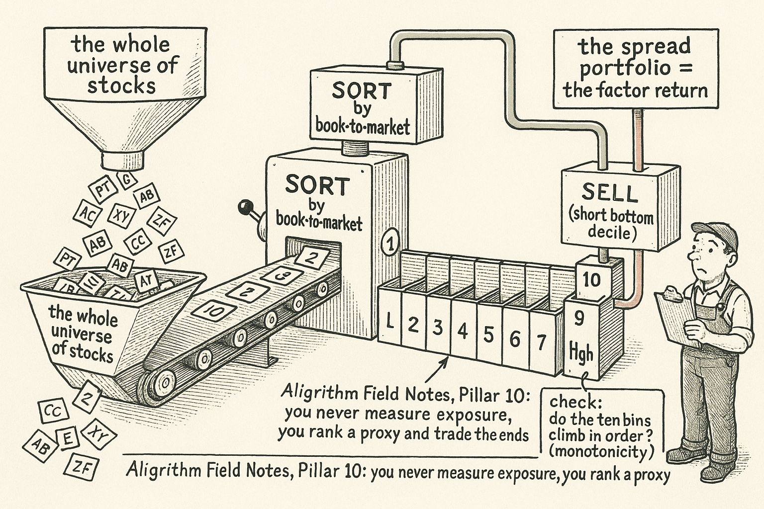
First, sorting. Fix a stock pool and rank every name in it by the sorting variable, high to low or low to high depending on whether the variable is positively or negatively related to return. Second, grouping. Cut the ranked list into L groups, and by convention L is 10, so you get deciles. Build a hedged portfolio by going long the top decile and shorting the bottom decile. That long-short book is the spread portfolio, and its return is your estimate of the factor return for that month. The two legs are dollar neutral, equal money long and short, and within each leg you weight stocks either equally or by market capitalization. Third, rebalance. A stock's book-to-market drifts over time, so you redo the sort on a schedule. Academics rebalance monthly or annually. Trading desks often rebalance a factor book daily, which sounds more diligent until you price in the turnover and the spread you pay on every name that crosses a decile boundary.

Notice what the spread portfolio quietly does. Going long the top and short the bottom nets out the exposures both groups share. If the whole market rallies, both legs rise and the move cancels. What is left is the return that specifically separates high book-to-market stocks from low ones, which is exactly the factor return you wanted and nothing else. That is the same neutralizing logic behind any ranked long-short book: the market move you cannot forecast gets subtracted by construction.

Is the spread real, or is it two lucky months

You now have a time series of monthly spread returns, one lambda per month. Testing whether the factor earns a premium is a t-test on that series, and it is the least glamorous, most load-bearing step in the whole pillar.

$$ \hat{\lambda} = \frac{1}{T}\sum_{t=1}^{T}\lambda_t, \qquad \text{se}(\hat{\lambda}) = \frac{\operatorname{std}(\lambda_t)}{\sqrt{T}}, \qquad t = \frac{\hat{\lambda}}{\text{se}(\hat{\lambda})} $$

Read it left to right. Lambda-hat is the average of your monthly spread returns, the estimated premium. The standard error is the sample standard deviation of those monthly returns divided by the square root of the number of months, which is just the standard error of a mean. The t-statistic is the premium divided by its standard error, and it follows a t-distribution with T minus 1 degrees of freedom. The minus one is there because you burned a degree of freedom estimating the standard deviation from the same sample.

Work the paper's own numbers. Sort Chinese stocks into ten book-to-market deciles, value-weight each decile, rebalance monthly. The high-minus-low spread averages 0.88% a month with a standard error of 0.47%. The t-stat is 0.88 divided by 0.47, which is 1.85, and the p-value is 0.07. That clears the 10% significance bar and nothing tighter. A 0.88% monthly premium sounds like a fortune, over 10% a year before costs, and the t-stat of 1.85 says you should hold your applause. It would not survive the multiple-testing tax that a later article covers, where the honest threshold for a factor dredged out of hundreds of candidates sits closer to a t of 3 than a t of 2. One sort, one barely-significant premium, is where the factor zoo's graveyard starts filling.

Monotonicity: the spread can lie

A positive high-minus-low spread is necessary and nowhere near sufficient. The number 0.88% is a difference between two endpoints, and two endpoints can look great while everything between them is garbage. Suppose deciles 1 through 9 are a flat, random mess and only the top decile spikes on a couple of lucky momentum names. The spread is still positive, the t-stat still prints, and you have a portfolio built on two data points pretending to be a monotone risk premium.

A real factor should explain the cross-section smoothly, so the ten decile returns should rise more or less in order as the sorting variable rises. The check is the rank correlation coefficient between the decile group labels and the decile returns.

$$ \rho_s = \frac{\operatorname{cov}(X_r, X_g)}{\sigma_{X_r}\,\sigma_{X_g}} $$

X_g is the group number, 1 through 10, and X_r is the rank of that group's average return, also 1 through 10. Rho-s is the ordinary correlation computed on those two sets of ranks, so it measures the monotonic relationship and ignores how big the gaps are. It runs from minus 1 to plus 1. A rho-s of plus 1 means the returns increase in perfect lockstep with the deciles, every step up in book-to-market buys a step up in return. Near zero means the ordering is noise and your spread is an accident at the ends.

Run it on the paper's deciles. The average returns from Low to High are 0.57, 0.53, 0.57, 0.72, 0.94, 0.90, 1.08, 1.32, 1.21, 1.44. Not a perfect staircase, decile 2 dips below Low and decile 6 slips under decile 5 and decile 9 under decile 8, but the trend up the ranking is unmistakable. Rank the returns, correlate against 1 through 10, and rho-s lands around 0.95. High, not perfect, which is what a genuine but noisy factor looks like.

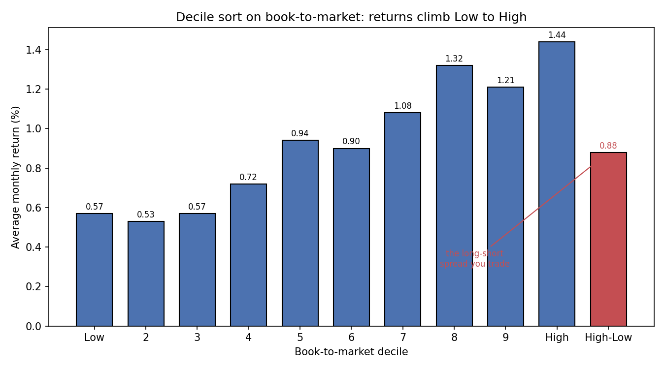
Bar chart of the ten book-to-market decile returns rising from Low to High, with the 0.88 percent high-minus-low spread shown as a separate red bar

The picture is the tell. A clean upward climb is what separates a factor from a fluke. If the bars looked like a flat field with one tall spike on the right, the spread would be the same 0.88% and the rank correlation would collapse, and you would know the premium is riding on a handful of names rather than a systematic pattern across the whole cross-section.

One sort controls nothing

Univariate sorting has a hole you can drive a truck through. Ranking on book-to-market alone gives you a portfolio that is long high book-to-market and short low book-to-market, but it does not check what else those two groups differ on. If high book-to-market stocks happen to be small caps and low book-to-market stocks happen to be large caps, your "value" spread is quietly also a long-small, short-large size bet. You wanted one factor and you built a blend of two, and you cannot tell how much of the 0.88% is value and how much is size leaking in.

The fix is to sort on two variables at once, double sorting. Cut the universe into L1 groups on the first variable and L2 groups on the second, giving L1 times L2 cells, and quintiles on each side are the common choice, so 25 portfolios. From that grid you build a factor for one variable by averaging across the other. For the first variable the return is the average of the top-X1 cells minus the average of the bottom-X1 cells:

$$ \lambda_{X_1,t} = \frac{1}{L_2}\sum_{i=1}^{L_2} R_{L_1 i,\,t} - \frac{1}{L_2}\sum_{i=1}^{L_2} R_{1 i,\,t} $$

The first sum runs across the whole top row of the grid, the high-X1 cells at every level of X2, and averages them. The second sum does the same for the bottom row, the low-X1 cells. Subtract, and X2 is averaged out of the picture, so the leftover is the X1 premium purged of X2. Concretely, with value as X1 and size as X2, you average value's spread across small, mid, and large stocks separately, so the size tilt cancels and you are left with a cleaner value premium.

Independent versus dependent, and why the cells go empty

Double sorting splits into two flavors, and the difference decides whether your grid is usable. Independent double sorting, also called unconditional, cuts each variable into quintiles using its own global breakpoints, then drops every stock into whatever cell its two ranks land in. Simple, symmetric, and it breaks the moment the two variables correlate.

If book-to-market and size move together in the cross-section, a high book-to-market stock is usually also small. Under independent breakpoints the stocks pile onto the diagonal of the grid, the high-high and low-low cells overflow while the off-diagonal cells, high on one variable and low on the other, run nearly empty. A cell holding six stocks is not a portfolio, it is a rounding error, and one outlier in it swings the whole factor return.

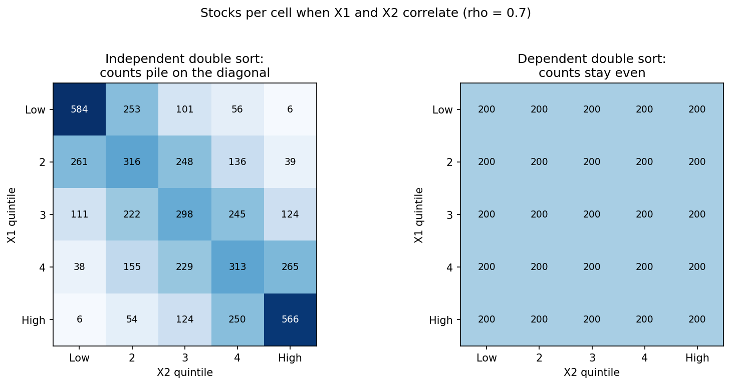
Two 5 by 5 grids of stock counts, the independent sort with counts piled on the diagonal and near-empty corners, the dependent sort with a flat 200 stocks in every cell

The left grid is the disease. Two correlated characteristics, and the corner cells hold hundreds of stocks while the opposite corners hold single digits. The right grid is the cure. Dependent double sorting, also called conditional, sorts on the first variable into L1 groups, then sorts on the second variable within each of those groups. Because the second cut happens inside each first-variable bucket, every cell gets the same count by construction, no empty corners, no outlier hostage situation.

Dependent sorting also answers a sharper question. It treats the two variables unequally on purpose. The first variable is a pure control, and the real question is whether the second variable still predicts returns after the first is held fixed. Does momentum add anything once you have already conditioned on size, or is it just size in disguise? A factor should be built only on the second, conditioned variable, because that is the one whose incremental information you just isolated. Independent sorting treats both variables as co-equal factors, dependent sorting treats the first as a nuisance you are controlling away, and knowing which you want is the difference between measuring a factor and measuring a confound.

Where this connects

The sort is the machine that produces lambda, and everything else in the pillar is a check on what comes out of it. The old article "What a Factor Actually Is" gave the equation; this article gave the estimator for its most slippery term. The premium test here, the t-stat on the mean spread, is the single-factor warm-up for the GRS test, which asks the same significance question about a whole vector of alphas at once. Fama-MacBeth, coming next, is the sort's regression-based cousin, estimating premiums in a second cross-sectional pass instead of a long-short book. And the barely-significant t of 1.85 on that value premium is the thread that leads straight into the factor zoo, where the reckoning is that most published sorts print a spread that dies the moment you correct for how many characteristics people tried.

Reach back too. The neutralizing logic of the spread portfolio, long the top and short the bottom so the shared exposure cancels, is the same move as the ranked long-short book from the Carver-side ranking articles and the cross-sectional percentile rank from the old article "Cross-Sectional Percentile Rank Within a Universe." Rank on a proxy, trade the ends, subtract what both ends share. The sort just makes that discipline exact enough to slap a t-stat on.

KEY POINTS

You never observe a stock's factor exposure or the factor premium. A portfolio sort ranks stocks on a measurable proxy like book-to-market and assumes only that the proxy is correlated with the true exposure, no functional form required.
The recipe is three steps: rank the universe on the sorting variable, cut into L groups (L equals 10 by convention), go long the top decile and short the bottom to form a dollar-neutral spread portfolio, then rebalance. The spread's monthly return is your estimate of the factor return.
Test the premium with a t-stat on the monthly spread returns: lambda-hat is the mean, the standard error is the standard deviation over the square root of the number of months, and the t-stat is the ratio on T minus 1 degrees of freedom.
The paper's book-to-market sort earns 0.88% a month with a t-stat of only 1.85 and a p-value of 0.07. That clears the 10% bar and nothing tighter, and it would not survive the multiple-testing correction a later article applies.
A positive high-minus-low spread can be two lucky endpoints. Check monotonicity with the rank correlation between decile number and decile return; a rho-s near 1 (about 0.95 in the example) means the returns climb smoothly with the ranking rather than spiking at one end.
Univariate sorting cannot control for other factors, so a value sort can secretly be a size bet. Double sorting cuts on two variables at once and averages one out to purge it from the other.
Independent double sorting uses global breakpoints and empties the off-diagonal cells when the two variables correlate, leaving factor returns hostage to outliers. Dependent double sorting sorts the second variable within each group of the first, keeps cell counts even, and isolates the second variable's incremental predictive power after controlling for the first.

References

- The Cross-Section of Expected Stock Returns (Fama and French, 1992)
- Common Risk Factors in the Returns on Stocks and Bonds (Fama and French, 1993)
- A Five-Factor Asset Pricing Model (Fama and French, 2015)
- Monotonicity in Asset Returns: New Tests with Applications to the Term Structure, the CAPM, and Portfolio Sorts (Patton and Timmermann, 2010)
- Digesting Anomalies: An Investment Approach (Hou, Xue, and Zhang, 2015)
- ... and the Cross-Section of Expected Returns (Harvey, Liu, and Zhu, 2016)
- Portfolio Sort Analysis, DDA3600: Factor Investing (Chuan Shi, 2024)
A note on AI. The ideas, research, analysis, and conclusions in this article are my own. I use AI tools to help with editing and wordsmithing, because English is not my first language, and I am not shy about that. AI-generated ideas and AI-assisted writing are not the same thing: the first is empty slop from a generic prompt, the second is a tool for communicating years of real research more clearly. Judge the work by its substance, not by whether software helped polish the prose.