10. Cross-Sectional & Factor Investing July 9, 2026 9 min

10.4 Fama-MacBeth Two-Pass and the Shanken Correction Nobody Applies

Fama-MacBeth gets you the factor premium in two passes, even for untradable factors. But the second pass uses estimated betas, so skipping the Shanken correction inflates every t-stat.

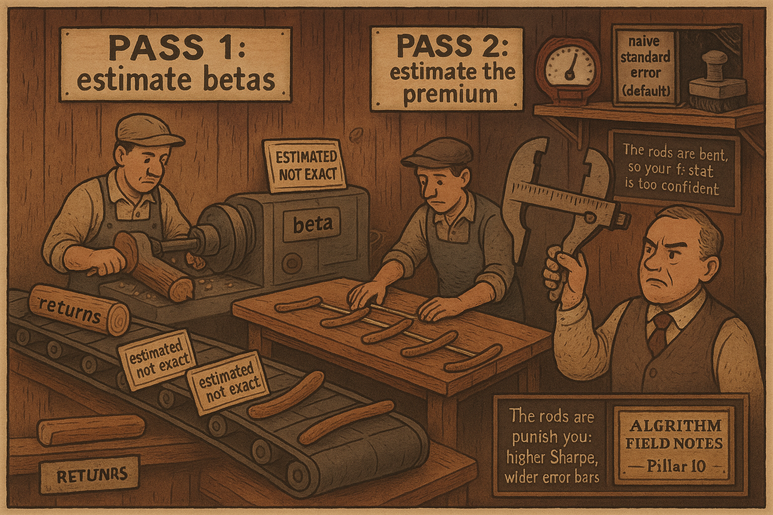
The old article "The GRS Test: Your Alpha Is Probably a Missing Factor" graded a model by running a time-series regression per asset and asking whether the alphas were jointly zero. That machine only works when your factors are tradable portfolios you can put on the right-hand side. Half the interesting factors are not. Industrial production, inflation surprises, a liquidity shock, an aggregate sentiment index: you cannot buy a share of GDP, so you cannot form its factor-mimicking portfolio and you cannot run the time-series test. You also often want a different thing from the test. GRS hands you a pass or fail on the whole model. Fama-MacBeth hands you the premium itself, a number with a t-stat, for each factor, tradable or not.

Fama-MacBeth is the most-run regression in empirical asset pricing. It is also the one whose standard errors are almost always reported wrong. The betas that go into the second pass were estimated in the first pass, and pretending they are known truth shrinks your standard errors and inflates your t-stats. Shanken wrote down the fix in 1992. Most practitioners still skip it, which is how a t of 1.99 gets published as a t of 2.3.

Two passes: betas first, premia second

Both cross-sectional methods share a first pass. Regress each asset's excess return on the factor returns over time to get its exposures, exactly as in the old article "The GRS Test: Your Alpha Is Probably a Missing Factor." That gives you beta-hat for every asset. The second pass is where the cross-sectional approach diverges: instead of reading the premium off a tradable factor's average return, you regress average returns across assets on their estimated betas.

$$ \mathbb{E}_T[R_i^e] = \hat{\beta}_i^\top \lambda + \alpha_i, \qquad \hat{\lambda} = (\hat{\beta}^\top \hat{\beta})^{-1}\hat{\beta}^\top \, \mathbb{E}_T[R^e] $$

Read it plainly. The left equation says each asset's long-run average excess return should equal its exposures times the factor premiums, and whatever is left over is the pricing error alpha-i. The right equation is just the OLS slope of that cross-sectional line: regress the vector of average returns on the matrix of betas, and the slope is lambda-hat, the estimated premium per unit of exposure. The line is fit to minimize the sum of squared pricing errors across assets.

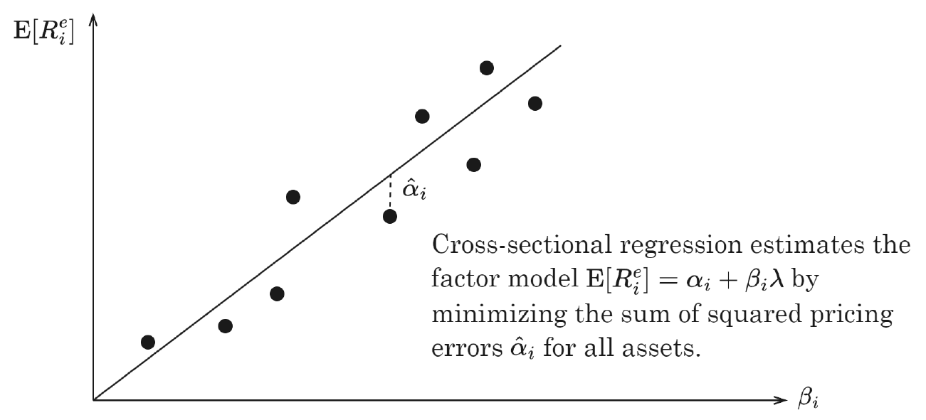
Scatter of average excess return against beta across assets with a fitted cross-sectional line, and alpha-i marked as the vertical distance of one asset from the line

Work a number. Suppose you have five test portfolios and, after the first pass, their market betas are 0.6, 0.8, 1.0, 1.2, 1.4, and their average monthly excess returns line up roughly on a line with slope 0.5% and a small scatter. The cross-sectional regression returns lambda-hat near 0.5% per unit of beta, so a portfolio with beta 1.2 is predicted to earn 0.6% a month. If it actually averaged 0.75%, its alpha is 0.15%, its distance above the line. The premium is the slope, the pricing errors are the residuals, and both fall out of one regression.

Fama-MacBeth: estimate then average

The plain cross-sectional regression runs once on the time-averaged returns. Fama-MacBeth flips the order. It runs the cross-sectional regression separately in every single period, producing a fresh premium estimate each month, then averages those estimates over time.

$$ \hat{\lambda} = \frac{1}{T}\sum_{t=1}^{T}\hat{\lambda}_t, \qquad \sigma(\hat{\lambda}_k) = \left[\frac{1}{T^2}\sum_{t=1}^{T}\left(\hat{\lambda}_{kt}-\hat{\lambda}_k\right)^2\right]^{1/2}, \qquad t = \frac{\hat{\lambda}_k}{\sigma(\hat{\lambda}_k)} $$

Each month t, regress that month's returns on the betas to get lambda-t, the factor's return that month. Average the lambda-t series to get the premium, and take its standard error the usual way for a mean: the standard deviation of the monthly estimates divided by the square root of T, which is why the sum carries one over T squared rather than one over T. The t-stat is the premium over its standard error. Plain cross-section averages first then estimates; Fama-MacBeth estimates first then averages. If the betas never changed over time the two give the identical premium, but in practice betas drift, and the original paper re-estimated them on a rolling window, using the beta known at t minus 1 to explain the return at t.

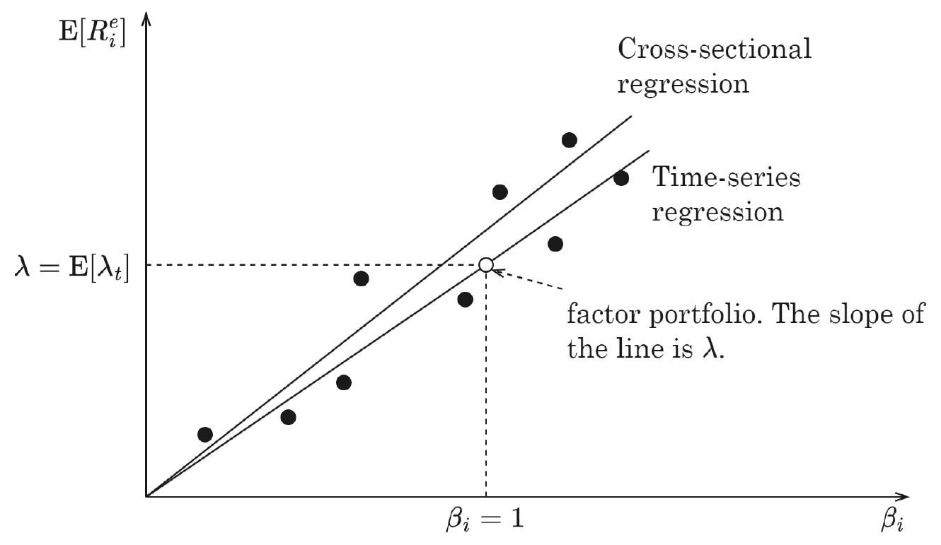
Two fitted lines on a plot of average return against beta, one from cross-sectional regression and one from time-series regression, meeting near the factor portfolio point at beta equal to one

The two lines are not the same line. The time-series line is pinned to run through the origin and the tradable factor portfolio, so its slope is forced to be the factor's own average return. The cross-sectional line is free to tilt and shift to minimize pricing errors across the test assets, so its slope can disagree with the factor's realized return. That freedom is the point when the factor is not tradable, and it is also the source of the problem in the next section. Fama-MacBeth's real advantage is that computing the premium period by period sidesteps the cross-sectional correlation among residuals that would wreck a single pooled regression's standard errors. Its weakness is that it assumes the monthly estimates are independent over time, which is why almost every modern paper layers a Newey-West adjustment on top to soak up autocorrelation.

The generated-regressor problem

Here is the crack everyone steps over. The second pass treats beta-hat as if it were the true beta. It is not. Beta-hat came out of a finite time-series regression in the first pass, so it carries sampling error, and now it sits on the right-hand side of the second regression as an explanatory variable. Regressing on a noisy regressor is the classic errors-in-variables problem. Two things happen. The premium estimate gets biased toward zero, because noise in a regressor flattens the slope. And, worse for anyone chasing significance, the naive standard error is too small, because it accounts for the scatter of returns around the line but ignores the scatter in the betas themselves.

The result is a t-stat that looks sturdier than it is. You did two estimation steps and only paid for the uncertainty in one. Every marginal factor whose t-stat sits between 2 and 3, exactly the band where the factor zoo lives, is a candidate to have its significance evaporate once you account for the first-pass noise.

The Shanken correction

Shanken derived the adjustment. The errors-in-variables piece of the premium's variance gets multiplied by a correction factor that depends on how good the factors are:

$$ \operatorname{cov}(\hat{\lambda}) \;=\; \frac{1}{T}\left[\left(1 + \hat{\lambda}^\top \hat{\Sigma}_f^{-1}\hat{\lambda}\right)\left(\hat{\beta}^\top\hat{\beta}\right)^{-1}\hat{\beta}^\top \Sigma \,\hat{\beta}\left(\hat{\beta}^\top\hat{\beta}\right)^{-1} + \hat{\Sigma}_f\right] $$

The term that matters is the multiplier one plus lambda-transpose Sigma-f-inverse lambda. That quantity, lambda-transpose Sigma-f-inverse lambda, is the maximum squared Sharpe ratio you can build from the factors per period. It is the same theta-squared that appears inside the GRS F-statistic from the old article "The GRS Test: Your Alpha Is Probably a Missing Factor." So the correction inflates the standard errors by the square root of one plus the factors' own squared Sharpe ratio. Good factors punish you: the more return-per-risk your factors already deliver, the more the correction widens your error bars on the premia estimated from them.

Put numbers on it. A plain three-factor model with an annual maximum Sharpe around 0.77 has a monthly squared Sharpe near 0.05, so the correction multiplies the variance by 1.05 and inflates the standard error by about 2.4%. Negligible. But take the composite four-factor model from the old article's China evidence, with an annual maximum Sharpe of 2.02. Its monthly squared Sharpe is about 0.34, the multiplier is 1.34, and the standard error inflates by about 16%. A premium that printed a t-stat of 2.3 with naive errors drops to roughly 1.99 once corrected, straight through the significance line.

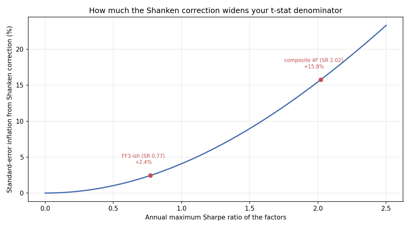
Curve showing standard-error inflation from the Shanken correction rising with the factors' annual Sharpe ratio, marked at 2.4 percent for a Sharpe of 0.77 and 15.8 percent for a Sharpe of 2.02

The curve is the whole argument for why this is not pedantry. For weak factors the correction rounds to nothing, which is why sloppy work survived for a while. For the high-Sharpe models that quant desks actually chase, it moves t-stats by enough to overturn a marginal discovery. Nobody applies it because the default output of every regression package is the uncorrected Fama-MacBeth standard error, and adding the multiplier takes an extra line of code plus an estimate of the factor covariance. The path of least resistance publishes the bigger t-stat.

Noisy betas also bias the premium, not just the error bar

The correction fixes the standard error, but the attenuation bias in the premium itself is a separate leak worth naming. Because beta-hat is measured with error, the estimated premium is dragged toward zero and the intercept is pushed up, so a real premium can look smaller than it is even as its significance looks larger than it is. Sorting stocks into portfolios before the second pass, the workhorse move from the old article "Portfolio Sorts From Scratch: Deciles, Monotonicity, and the Long-Short Spread," is partly a defense against this: a portfolio's beta is averaged over many stocks, so it is estimated far more precisely than any single stock's beta, and the errors-in-variables damage shrinks. The cost is that you throw away cross-sectional spread by collapsing thousands of stocks into ten or twenty-five buckets. Precise betas or a wide cross-section, and you rarely get both.

Where this connects

Fama-MacBeth is the cross-sectional twin of the time-series GRS test from the old article "The GRS Test: Your Alpha Is Probably a Missing Factor." GRS forces the model through tradable factor portfolios and tests the alphas jointly; Fama-MacBeth estimates the premium directly, tradable factor or not, and tests it with a t-stat. The pricing error alpha-i is the same object in both, and it is the same object as the residual return in the old article "Predict Residual Returns, Not Gross." That article argued you should forecast the idiosyncratic leftover after stripping the factors; the Fama-MacBeth second pass is how you measure what each unit of exposure earned so you know exactly what to strip. Estimate the premia, subtract beta times premium, and forecast only what survives.

The Shanken correction is one more reason the honest significance bar sits higher than the reflexive t of 2. Between generated-regressor noise, the correction most people skip, and the multiple-testing tax across hundreds of candidate factors, a premium needs a lot more than a naive t of 2 to be real. That reckoning gets its own article on the factor zoo.

KEY POINTS

Fama-MacBeth is a two-pass estimator: first estimate each asset's betas from time-series regressions, then regress average returns on those betas across assets to get the factor premium. It works even when the factor is not a tradable portfolio, which the time-series GRS test cannot handle.
The second pass fits a cross-sectional line whose slope is the premium lambda and whose residuals are the pricing errors alpha. The line minimizes squared pricing errors across the test assets.
Fama-MacBeth runs the cross-sectional regression every period and averages the resulting premium estimates, so its standard error is the standard deviation of the monthly estimates over the square root of T. This sidesteps cross-sectional residual correlation but assumes no time-series autocorrelation, which Newey-West patches.
The betas fed into the second pass were estimated in the first pass, so they carry noise. This errors-in-variables problem biases the premium toward zero and makes the naive standard error too small, inflating t-stats.
The Shanken correction multiplies the errors-in-variables part of the premium variance by one plus the factors' own maximum squared Sharpe ratio, the same theta-squared that appears in the GRS F. Standard errors inflate by the square root of that factor.
The correction is tiny for weak factors (about 2% for an annual Sharpe of 0.77) but large for high-Sharpe models (about 16% for the composite four-factor model's Sharpe of 2.02, enough to drop a t of 2.3 to 1.99). Nobody applies it because uncorrected errors are the default output.
Sorting into portfolios before the second pass averages betas over many stocks, cutting the errors-in-variables damage, at the cost of collapsing cross-sectional spread.

References

- On the Estimation of Beta-Pricing Models (Shanken, 1992)
- Risk, Return, and Equilibrium: Empirical Tests (Fama and MacBeth, 1973)
- A Test of the Efficiency of a Given Portfolio (Gibbons, Ross, and Shanken, 1989)
- Common Risk Factors in the Returns on Stocks and Bonds (Fama and French, 1993)
- A Simple, Positive Semi-Definite, Heteroskedasticity and Autocorrelation Consistent Covariance Matrix (Newey and West, 1987)
- Size and Value in China (Liu, Stambaugh, and Yuan, 2019)
- Regression-Based Test, DDA3600: Factor Investing (Chuan Shi, 2024)
A note on AI. The ideas, research, analysis, and conclusions in this article are my own. I use AI tools to help with editing and wordsmithing, because English is not my first language, and I am not shy about that. AI-generated ideas and AI-assisted writing are not the same thing: the first is empty slop from a generic prompt, the second is a tool for communicating years of real research more clearly. Judge the work by its substance, not by whether software helped polish the prose.