10. Cross-Sectional & Factor Investing July 9, 2026 10 min

10.3 The GRS Test: Your Alpha Is Probably a Missing Factor

Alpha is the gap between what a portfolio earned and what your model predicts. The GRS test grades all those gaps at once, and the usual verdict is blunt: you are missing a factor.

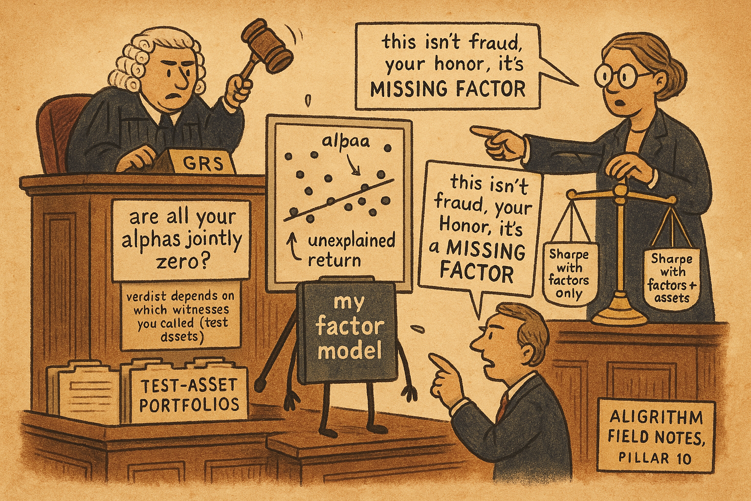
The old article "Portfolio Sorts From Scratch: Deciles, Monotonicity, and the Long-Short Spread" left you with one spread portfolio and one t-stat on its average return. That is fine when you have a single factor to judge. But the real question a factor model faces is not "does this one spread pay," it is "does my model price everything at once." You hand the model a whole panel of test portfolios, twenty-five size-and-value cells, ten momentum deciles, whatever, and you ask whether it leaves any of them with a return it cannot explain. Every leftover is an alpha, and a model that prices the cross-section should leave all of them at zero together.

Alpha here is not a bragging number. It is the pricing error, the vertical gap between what a portfolio actually earned and what the model says it should have earned given its exposures. A significant alpha means one of three things: the asset is genuinely mispriced, you got unlucky with a small sample, or, most of the time, your model is missing a factor that the asset happens to load on. The Gibbons-Ross-Shanken test is the one number that grades all the pricing errors jointly, and it usually delivers the same verdict: your alpha is a factor you forgot to include.

Alpha is the gap, not the glory

Start with the workhorse. For each test asset you run a time-series regression of its excess return on the factor returns, month by month:

$$ R_{it}^e = \alpha_i + \beta_i^\top \lambda_t + e_{it}, \qquad t = 1, 2, \cdots, T $$

Read it left to right. The excess return of asset i in month t equals a constant alpha, plus the asset's exposures beta-transpose times the factor returns that month, plus a shock. Run OLS and you get two things per asset: beta-i, how much of each factor it carries, and alpha-i, the part of its average return the factors never touched. Average over time and the model's prediction for the asset is beta-transpose times the average factor premium, so alpha is whatever sits above or below that prediction. On a plot of average return against beta, the model is a straight line and alpha is the height of the asset above the line.

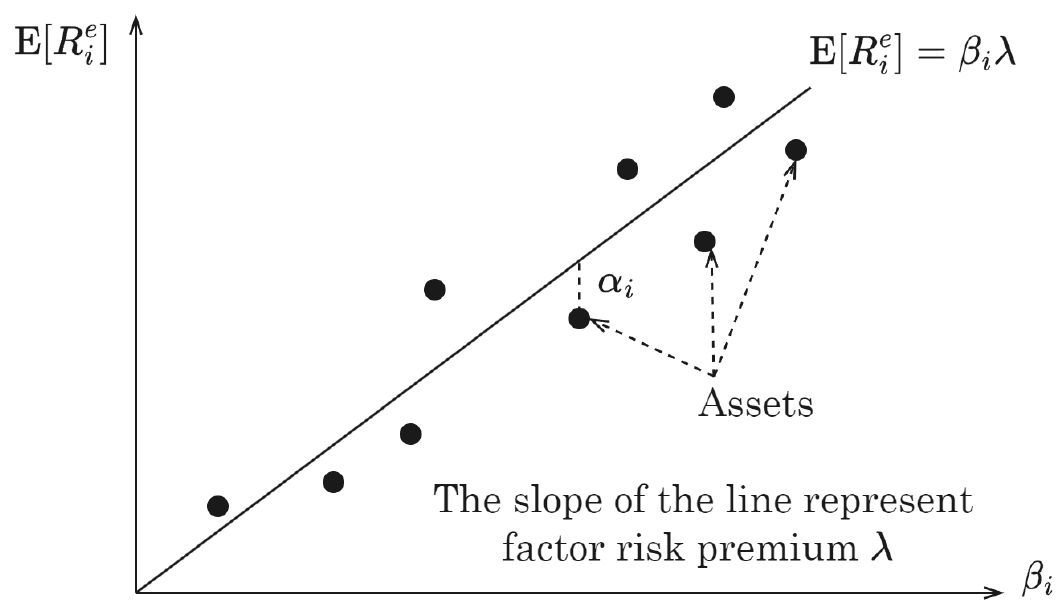
Scatter of average excess return against beta with the factor model drawn as a straight line, and alpha-i marked as the vertical distance from an asset up to the line

The dots that sit off the line are the model's failures. Work a number. Say a value portfolio averaged 1.2% a month, its market beta is 1.5, and the market premium averaged 0.6% a month. The single-factor model predicts 1.5 times 0.6, which is 0.9%. The portfolio earned 1.2%, so its alpha is 0.3% a month of return the market factor never accounted for. That 0.3% is either a genuine anomaly, noise, or a signal that a value factor belongs in the model. The regression alone will not tell you which, and that ambiguity is the whole game.

One test per asset lies, so test them jointly

You could eyeball each alpha and its own t-stat, but that road leads straight into the multiple-testing trap the old article "Portfolio Sorts From Scratch: Deciles, Monotonicity, and the Long-Short Spread" flagged. Run twenty-five separate t-tests at the 5% level and you expect one or two to print significant by chance even if every true alpha is zero. The fix is to test the entire vector of alphas in one shot. Stack them into alpha equals the column of alpha-1 through alpha-N, and ask whether that whole vector is jointly zero.

The natural statistic is a quadratic form: the alpha vector, squeezed through the inverse of its own covariance matrix, back against itself.

$$ \hat{\alpha}^\top \, \operatorname{cov}(\hat{\alpha})^{-1} \, \hat{\alpha} \; \sim \; \chi^2_N $$

The middle term weights each pricing error by how precisely it was estimated and how the errors move together, so a big alpha on a noisy, correlated portfolio counts for less than a modest alpha on a clean, independent one. Under the null that all alphas are zero, this quadratic form follows a chi-squared distribution with N degrees of freedom, one for each test asset. Large value, small p-value, reject the model. That is the asymptotic version, and it leans on having a long sample T for the central limit theorem to bite.

The GRS F-statistic

Gibbons, Ross, and Shanken took one more step in 1989. Instead of the large-sample chi-squared approximation, they derived the exact small-sample distribution of the scaled pricing errors, which turns out to be an F:

$$ \frac{T-N-K}{N}\left(1 + \hat{\theta}^2\right)^{-1}\,\hat{\alpha}^\top \hat{\Sigma}^{-1}\hat{\alpha} \;\sim\; F_{N,\,T-N-K} $$

Take it apart. Alpha-transpose Sigma-inverse alpha is the size of the pricing errors, scaled by the residual covariance Sigma, so correlated residuals do not get double-counted. The term one over one-plus-theta-squared is a correction for how good the factors themselves are, where theta is the factors' own Sharpe ratio, and more on that in a second. The fraction (T minus N minus K) over N converts the whole thing into an F statistic with N and T-minus-N-minus-K degrees of freedom, where K is the number of factors. The F distribution is exact for finite T, which matters because asset-pricing samples are short. Twenty years of monthly data is only 240 observations, and the chi-squared approximation is optimistic at that length.

The verdict is a single p-value on the null that the model prices everything. The China data in the deck shows both outcomes cleanly. Test the two Fama-French factors as assets against the Chinese three-factor model and the GRS F is 0.88 with a p-value of 0.41, so you cannot reject, the Chinese model prices the imported factors. Reverse it, test the Chinese size and value factors against Fama-French, and the GRS F is 33.90 with a p-value of 2.14 times ten to the minus thirteen. That is not a close call. Fama-French leaves the Chinese factors with alphas so large the model is rejected into the ground.

What GRS is really measuring: a Sharpe-ratio gap

The F formula looks like bookkeeping until you rewrite it. The same statistic equals a comparison of two Sharpe ratios:

$$ \frac{T-N-K}{N}\left(\frac{1+\hat{\theta}_{N+K}^2}{1+\hat{\theta}_K^2} - 1\right) \;\sim\; F_{N,\,T-N-K} $$

Here theta-K squared is the maximum squared Sharpe ratio you can build from the K factors alone, and theta-(N+K) squared is the maximum squared Sharpe ratio from the factors plus all N test assets. GRS is asking one question: do the test assets let you build a materially better tangency portfolio than the factors already give you? If the factors span everything worth spanning, adding the test assets barely nudges the Sharpe ratio, the ratio sits near one, the statistic is small, and the model survives. If the test assets open up a much steeper Sharpe frontier, the factors are missing something, the alphas are real, and GRS rejects.

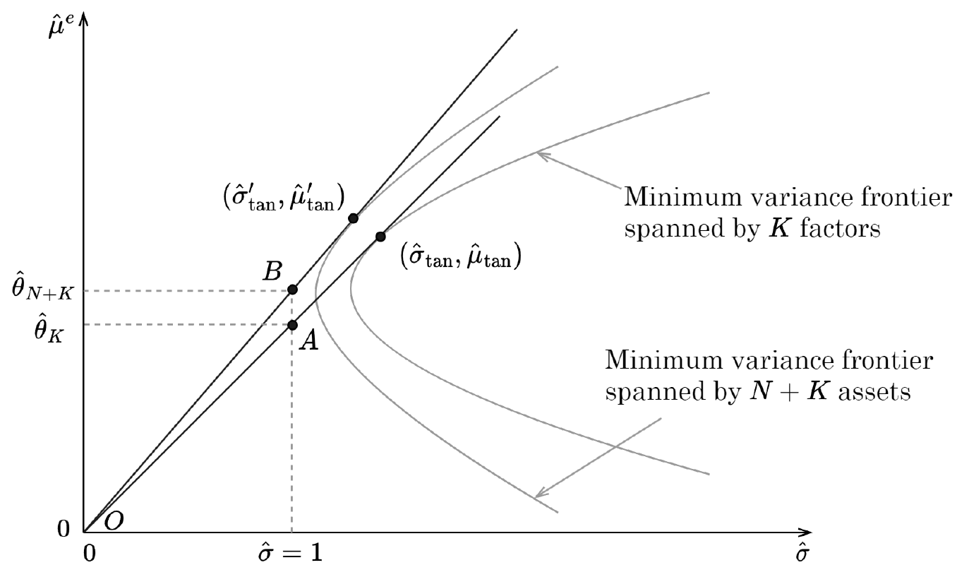
Two minimum-variance frontiers on a return-versus-risk plot, the outer one spanned by factors plus test assets reaching a higher tangency Sharpe ratio than the inner one spanned by the factors alone

The picture is the argument. The inner frontier is what the factors can reach, the outer frontier is what factors plus assets can reach, and the gap between the two tangency lines is exactly what GRS measures. This is why the test is really a factor-completeness check. The deck reports the maximum annual Sharpe ratio spanned by three competing models: a composite four-factor model reaches 2.02, Stambaugh-Yuan reaches 0.98, and Daniel-Hirshleifer-Sun reaches 0.80. A model whose factors already span a Sharpe of 2.02 leaves little room for test assets to improve on it, so it will reject far fewer of them. The higher your factors' own Sharpe ratio, the harder it is for any anomaly to show a significant alpha against you.

Your alpha is probably a missing factor

Now the title earns itself. A big alpha against your model is rarely free money. Feed one model's factors in as the other model's test assets and the pattern is stark. Against the Chinese three-factor model, the Fama-French value factor carries an alpha of 0.34 with a t-stat of 0.97, statistically indistinguishable from zero, and the Fama-French size factor an alpha of minus 0.04 with a t-stat of minus 0.66. The Chinese model spans them; they add nothing it does not already have. Run it the other way and the Chinese value-minus-growth factor shows an alpha of 1.39 with a t-stat of 7.93 against Fama-French, and the Chinese size factor an alpha of 0.47 with a t-stat of 7.03. Those enormous alphas are not evidence that China prints free returns. They are evidence that Fama-French is missing the factor the Chinese model built.

That is the joint-hypothesis problem from the old article "What a Factor Actually Is: α + βλ, and Why the Market Is Factor #1," made operational. A nonzero alpha says the market is inefficient or your model is wrong, and the test cannot separate the two. GRS does not break that tie. It quantifies how badly your current model fails, which almost always gets fixed by adding a factor rather than declaring the market broken. The lazy academic move is to keep bolting on factors until every alpha vanishes in-sample, which is curve-fitting with a respectable vocabulary, and it manufactured a large share of the factor zoo that a later article tears apart.

The test-asset trap

GRS has a soft underbelly, and the deck names it. The entire verdict depends on which test assets you feed it. Swap the test portfolios and the same model can pass one gauntlet and fail another, because you are only ever asking whether the model prices these particular assets. Nothing stops a researcher from quietly choosing the test assets that flatter their own model, which is data snooping wearing a lab coat. Worse, adding a factor to a model can sometimes raise the pricing errors on a given set of test assets rather than lower them, so "more factors" is not monotonically "better model."

There is one honest use of GRS for model comparison: count how many test assets still show a significant alpha against each model. Fewer survivors means the model prices more of the cross-section.

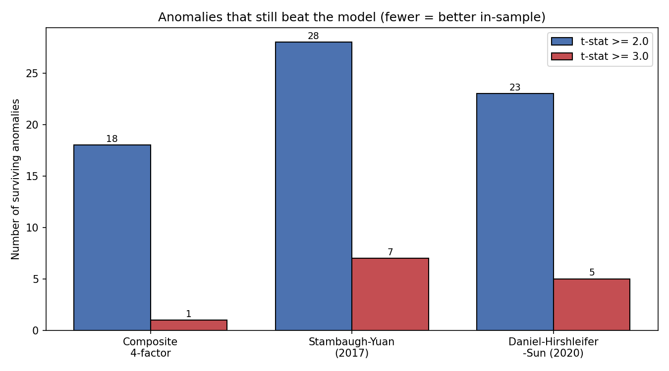
Grouped bar chart of the number of anomalies that still show a significant alpha against three factor models, at t-stat thresholds of 2.0 and 3.0, with the composite four-factor model leaving the fewest

The composite four-factor model leaves 18 anomalies alive at a t-stat above 2.0 and only 1 above 3.0, against 28 and 7 for Stambaugh-Yuan and 23 and 5 for Daniel-Hirshleifer-Sun. By this scoreboard the composite model wins. But read the gap between the two thresholds. Raising the bar from a t of 2.0 to a t of 3.0 collapses the survivor count for every model, which is the whole multiple-testing reckoning in one picture. Most of those t-between-2-and-3 anomalies are noise dressed as discovery, and the honest threshold in a field that tested hundreds of signals is closer to 3 than 2. That fight gets its own article. And every number here is in-sample; none of it promises the model prices anything out of sample, which is where factor claims go to die.

Where this connects

GRS is the joint version of the single t-stat from the old article "Portfolio Sorts From Scratch: Deciles, Monotonicity, and the Long-Short Spread." One sort gives you one premium and one t-test; a whole panel of sorts gives you a vector of alphas and needs GRS. The next step, the two-pass Fama-MacBeth regression, attacks the same panel from the other direction, estimating premiums cross-section by cross-section instead of asset by asset, and it comes with the Shanken correction almost nobody applies.

It also lands on the same point as the old article "Why Benchmarks Matter in Rule Evaluation." A rule's return means nothing until you net it against the right benchmark, and alpha is exactly that: return minus what the model already explains. GRS just does the netting for a whole book of portfolios at once and asks whether anything survives. Pick a weak benchmark and everything looks like alpha; pick the right factor model and most of your edge turns out to be exposure you already owned.

KEY POINTS

Alpha is the pricing error, the gap between what a test asset earned and what the model predicts from its exposures. A significant alpha usually means the model is missing a factor, not that you found free money.
Testing alphas one asset at a time invites false positives across many portfolios. GRS tests the whole vector of alphas jointly, so a model that prices the cross-section leaves every pricing error at zero together.
The joint quadratic form alpha-transpose times the inverse covariance times alpha follows a chi-squared with N degrees of freedom asymptotically. Gibbons-Ross-Shanken sharpened this into an exact small-sample F with N and T-minus-N-minus-K degrees of freedom, which matters because asset-pricing samples are short.
GRS is really a Sharpe-ratio comparison: it asks whether the test assets build a materially higher maximum Sharpe ratio than the factors alone. A model whose factors already span a high Sharpe (the composite model reaches 2.02 annual) rejects far fewer anomalies.
Worked verdict from the China data: the Chinese three-factor model prices the Fama-French factors (GRS F 0.88, p 0.41), but Fama-French fails badly on the Chinese factors (GRS F 33.90, p about ten to the minus thirteen; value-minus-growth alpha 1.39, t 7.93). The huge alpha is a missing factor.
The verdict depends entirely on the choice of test assets, which opens the door to data snooping, and adding a factor can even raise pricing errors on a given test set. More factors is not automatically a better model.
Counting surviving anomalies is a fair model-comparison scoreboard, but raising the bar from t above 2 to t above 3 collapses every model's survivor count, and it is all in-sample. The out-of-sample test is where factor claims usually break.

References

- A Test of the Efficiency of a Given Portfolio (Gibbons, Ross, and Shanken, 1989)
- Common Risk Factors in the Returns on Stocks and Bonds (Fama and French, 1993)
- A Five-Factor Asset Pricing Model (Fama and French, 2015)
- Digesting Anomalies: An Investment Approach (Hou, Xue, and Zhang, 2015)
- Size and Value in China (Liu, Stambaugh, and Yuan, 2019)
- ... and the Cross-Section of Expected Returns (Harvey, Liu, and Zhu, 2016)
- Regression-Based Test, DDA3600: Factor Investing (Chuan Shi, 2024)
A note on AI. The ideas, research, analysis, and conclusions in this article are my own. I use AI tools to help with editing and wordsmithing, because English is not my first language, and I am not shy about that. AI-generated ideas and AI-assisted writing are not the same thing: the first is empty slop from a generic prompt, the second is a tool for communicating years of real research more clearly. Judge the work by its substance, not by whether software helped polish the prose.