10. Cross-Sectional & Factor Investing July 9, 2026 9 min

10.6 Does ML Actually Help Asset Pricing? Kelly's 20%, Not 2–3×

ML promises to triple your Sharpe. Bryan Kelly, who builds the models, says expect 20%. Headline numbers die under fair tests, 166% turnover, and alpha trapped in tiny illiquid stocks.

The pitch writes itself. Feed a neural network four hundred firm characteristics, let it learn the nonlinear interactions that linear factor models miss, and watch the out-of-sample Sharpe ratio jump. The published tables cooperate: a random forest at 2.19, a neural network at 3.21, an IPCA model at 3.39, against a Fama-French three-factor Sharpe closer to 0.5. Read those numbers straight and machine learning looks like it quadruples your risk-adjusted return.

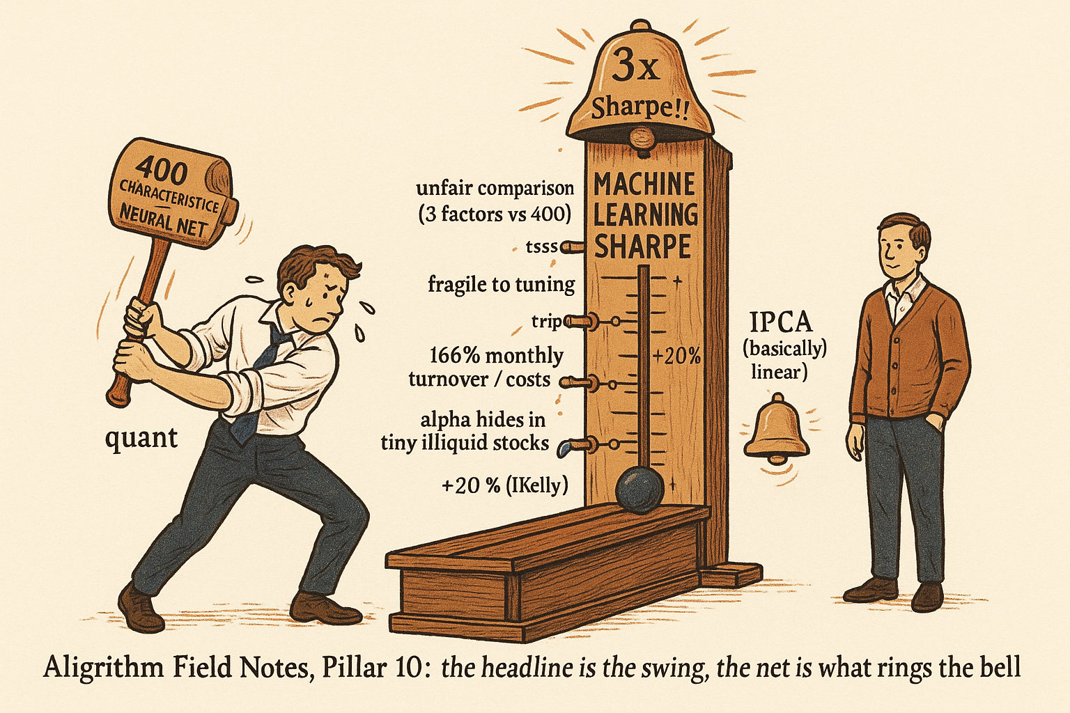
Then listen to Bryan Kelly, who builds these models for a living. His own words: you should not expect machine learning to double or triple your Sharpe ratio, and a 20 percent bump from adding nonlinearities feels realistic to him. That gap, between the 2-to-3x the tables imply and the 20% the practitioner will admit to, is the whole story. This deck by Chuan Shi is a facts-and-fictions teardown of machine learning in factor investing, and the honest verdict is that ML helps at the margin while the headline numbers are a magic trick built on unfair comparisons, fragile tuning, and untradable stocks. It is the same discipline as the old article "Optimization Comes After Testing, Not Before": the impressive first number is never the deployable number.

The evaluation has to survive itself

Before you believe any machine-learning Sharpe, ask how it was validated, because the validation protocol decides whether the number means anything. Plain k-fold cross-validation shuffles the data into folds and assumes the observations are independent. Financial data is not independent. Consecutive months are correlated, so a fold that trains on month t and tests on month t plus one lets the model learn the answer through the back door. Walk-forward respects time order but gives you exactly one path through history, one lucky or unlucky sequence, and no distribution to judge it against.

Combinatorial purged cross-validation, from Lopez de Prado, fixes both. Split the sample into N blocks, use K of them for testing, and enumerate every way to choose those K blocks.

$$ \text{number of backtest paths} = \binom{N}{K} $$

The count is the binomial coefficient, N choose K, the number of distinct test groups you can form. Work it with the deck's example: N equal to 6 blocks and K equal to 2 gives 6 choose 2, which is 15 backtest paths instead of one. Each path trains on the other blocks, with a purge buffer deleting the observations adjacent to the test blocks so no correlated neighbor leaks across the boundary. Now you have a distribution of 15 out-of-sample Sharpes, and you can ask whether the median is any good rather than betting on a single draw. This is the cross-sectional cousin of the overfitting diagnostics from Pillar 3, and it is the first filter any ML result has to pass.

The penalized-regression zoo is priors with a dial

Most of what gets sold as machine learning in asset pricing is regularized linear regression. You take the OLS objective and bolt on a penalty that punishes large coefficients.

$$ \min_{\beta_1,\dots,\beta_K} \sum_{i=1}^{N}\left(y_i - \beta_0 - \beta_1 x_{1i} - \cdots - \beta_K x_{Ki}\right)^2 + \lambda \sum_{j=1}^{K} f(\beta_j) $$

The first term is ordinary least squares, the sum of squared prediction errors. The second term is the penalty, lambda times a function of the coefficients, and the intercept is deliberately left out of it. Lambda is the dial. Set the penalty function to the sum of squared coefficients and you get ridge regression; set it to the sum of absolute values and you get the lasso, which drives weak coefficients exactly to zero and performs variable selection for free. Worked at the extremes: as lambda goes to zero the penalty vanishes and you are back to plain OLS, and as lambda goes to infinity every coefficient is crushed to zero and the model predicts the mean. Everything useful happens in between, and validation picks the spot.

The honest way to read this is Bayesian, and the deck says so. Ridge is what you get when you put a normal prior centered at zero on the coefficients, and the ridge lambda is precisely the ratio of noise variance to prior variance, sigma-squared over sigma-zero-squared. The lasso is the same idea with a Laplace prior, which has a spike at zero and so produces sparsity. There is no magic here. Penalized regression is you telling the model, before it sees the data, that most characteristics probably do not matter much, and then letting the data argue you out of it. On the deck's own test, 54 characteristics on the CSI 500 with a rolling 36-month window, the elastic net beat OLS out of sample. Real, useful, and about as revolutionary as admitting you have a prior.

The nonlinear end: autoencoders and an adversarial SDF

The genuinely nonlinear models are where the 2-to-3x dream lives. A conditional autoencoder, from Gu, Kelly, and Xiu, lets factor exposures move: instead of a static beta, the loading on each latent factor becomes a neural-network function of the firm's characteristics, so a stock's risk profile updates as its fundamentals change. The deepest version is the adversarial approach of Chen, Pelger, and Zhu. Start from the no-arbitrage condition, that the stochastic discount factor prices every excess return to zero, and turn model-building into a fight.

$$ \min_{w}\ \max_{g}\ \frac{1}{N}\sum_{j=1}^{N}\left\|\ \mathbb{E}\!\left[\left(1 - \sum_{i=1}^{N} w(I_t, I_{i,t})\, R^e_{i,t+1}\right) R^e_{i,t+1}\, g(I_t, I_{i,t})\right]\right\|^2 $$

Read it as a zero-sum game. The inner term is a pricing error: one minus the SDF's weighted returns, multiplied by a test-asset return built by the function g. One network, w, plays the asset pricer and tries to minimize those pricing errors. The adversary network, g, plays the attacker and searches for the managed portfolios where the SDF fails worst, maximizing the error. They iterate: the attacker finds the most mispriced corner of the market, the pricer patches it, repeat until the attacker cannot find a big miss. On Chen and coauthors' numbers this genuinely wins, a test Sharpe of 0.75 for the GAN model against 0.44 for a plain feed-forward network and 0.50 for the elastic net, with the highest cross-sectional R-squared of the batch at 0.23. So nonlinearity does add something real. The question is how much of it you keep.

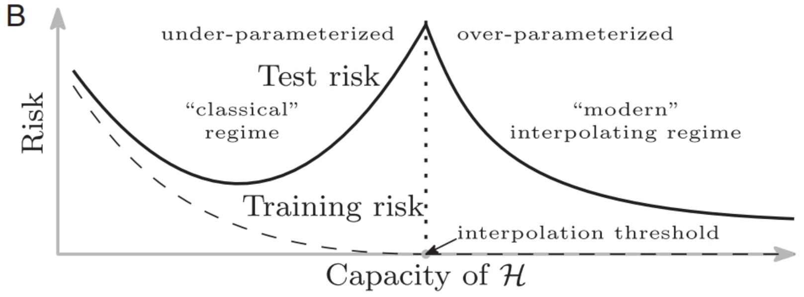
Classic double-descent curve: test risk falls, rises to a peak at the interpolation threshold, then falls again in the over-parameterized regime, while training risk decays monotonically

The theoretical cover for going complex is double descent. The old bias-variance story says test error rises once a model has more parameters than it can justify. The modern picture, from Belkin and coauthors, adds a second descent: push past the interpolation threshold, where the model has enough capacity to fit the training data exactly, and test error can fall again. Over-parameterized models can generalize. Fine. But asset-pricing data has a signal-to-noise ratio near the floor and a data-generating process that will not sit still, so the second descent is a much dicier bet here than in image recognition.

The headline Sharpes are a magic trick

Now the teardown. Three things inflate the published numbers. First, the comparison is rigged: the machine-learning model gets hundreds of characteristics while the Fama-French benchmark gets three, so of course the kitchen sink wins. Give both the same information and the gap shrinks. Second, the results are fragile. Re-evaluate the same models carefully and the Sharpes fall hard.

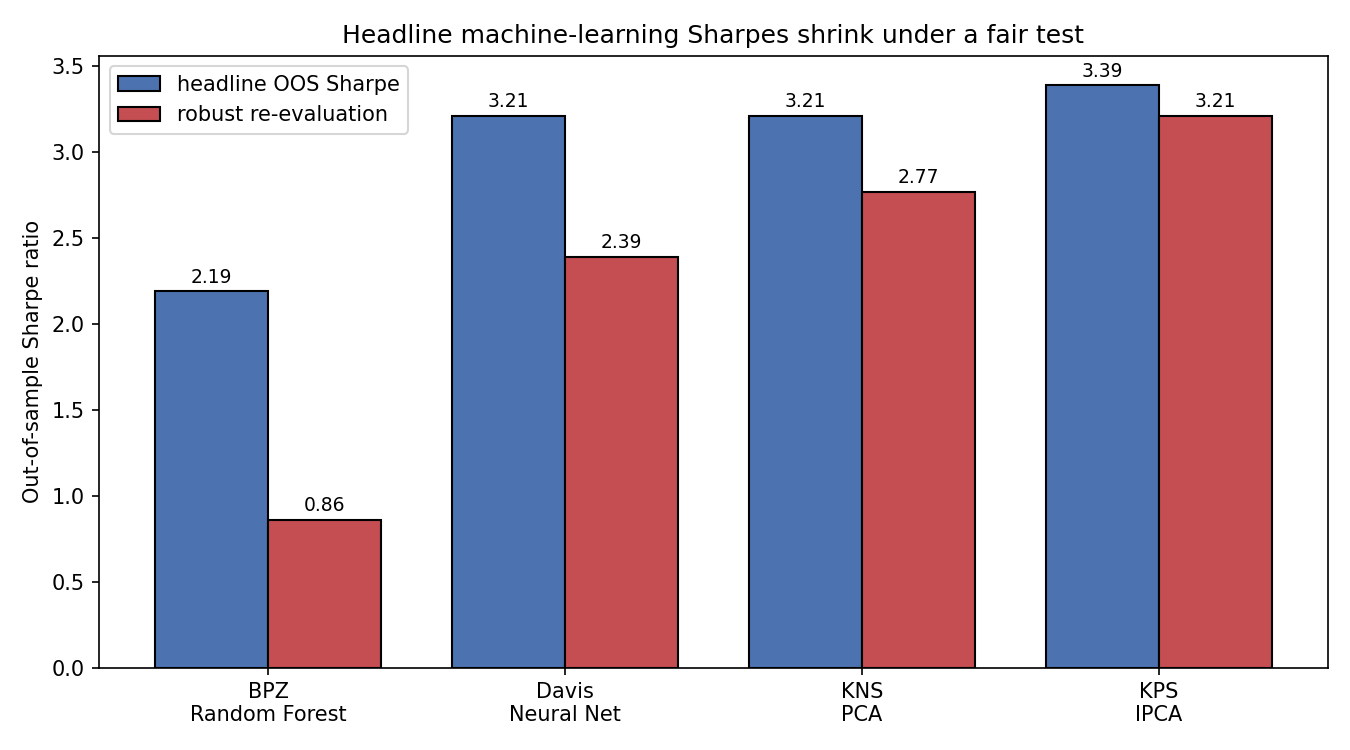
Grouped bar chart of headline versus robust out-of-sample Sharpe ratios for four models, with the random forest collapsing from 2.19 to 0.86 and the linear IPCA barely moving from 3.39 to 3.21

The random forest headline of 2.19 becomes 0.86 under a fair test, a 61% haircut. The neural network drops from 3.21 to 2.39. The one model that barely flinches is IPCA, from 3.39 to 3.21, and IPCA is essentially a linear model, characteristics-as-covariances estimated by cross-sectional regression. The most linear method is the most robust and finishes on top. That is the opposite of the ML-doubles-your-Sharpe story. Third, and this is Kelly's point stated as math, linear models are the first-order approximation and first-order approximations capture most of the signal, so nonlinearity is a second-and-third-order correction. A 20% Sharpe improvement is a good result. Expecting 200% is expecting the correction terms to dwarf the main term, which is not how good approximations work.

The untradable fine print

Suppose the gain survives all that. You still have to trade it, and here the machine-learning portfolios fall apart. Their edge comes from constant rebalancing.

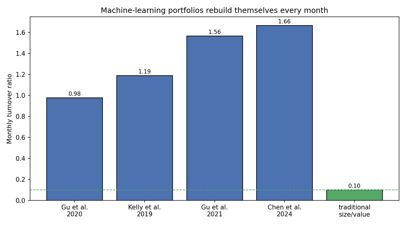
Bar chart of monthly turnover: machine-learning models between 0.98 and 1.66, against traditional size and value factors at roughly 0.10

The turnover numbers from Avramov and coauthors are brutal: the Gu-Kelly-Xiu model turns over 98% of the book every month, Kelly-Pruitt-Su 119%, the autoencoder 156%, the Chen-Pelger-Zhu GAN 166%. Traditional size and value factors sit below 10%. A model that rebuilds itself every month is paying spreads and impact ten to sixteen times as often as a value sleeve. At a rough 30 basis points round-trip cost, 100% monthly turnover is about 3.6% a year in frictions, enough to swallow the entire nonlinear premium (that cost figure is a back-of-envelope, flag it as illustrative). Worse, the deck's Fact 5 shows where the predictability lives: in the short legs and the tiny, illiquid, distressed, unrated stocks. Exclude the microcaps and the nonlinear models decline sharply while IPCA stays consistent across the full sample and the subsamples. The alpha is concentrated exactly in the names an institution cannot short cheaply or size into. On paper it is real. In a fund it is a rumor.

Where this connects

This is the same lesson the old article "Optimization Comes After Testing, Not Before" taught in the time-series world, transplanted to the cross-section. There the trap was a team polishing an in-sample Sharpe of 1.4 that evaporated on deployment. Here the trap is a published out-of-sample Sharpe of 3.2 that halves under a fair comparison and dies after costs. Combinatorial purged cross-validation plays the role the parameter-stability map played there: it turns one flattering number into a distribution you can be skeptical about. The machine-learning arc that runs through the Idea 3 articles on regression trees, random forests, and gradient boosting supplies the algorithms; this article supplies the reason to distrust their brochure.

The next question is when the complexity is actually worth paying for. Global models trained on 24 markets and dozens of characteristics can beat local ones, but only when there is enough data to feed the extra parameters, and linear methods still slightly prefer staying local. That data-hunger-versus-complexity tradeoff is the subject of the global-versus-regional article to come.

KEY POINTS

The headline pitch is that machine learning multiplies your Sharpe ratio 2-to-3x. Bryan Kelly, who builds these models, says expect about 20% from nonlinearity, not 200%. That gap is the entire argument.
Validate before you believe. K-fold assumes independent data and leaks through correlated neighbors; walk-forward gives one path. Combinatorial purged cross-validation enumerates N-choose-K test groups (15 paths for N=6, K=2) with a purge buffer, turning one Sharpe into a distribution.
Most ML in asset pricing is penalized regression: OLS plus a lambda-weighted coefficient penalty. Ridge is a Gaussian prior with lambda equal to noise-to-prior variance ratio; the lasso is a Laplace prior that zeroes weak coefficients. It is priors with a dial, not magic.
The nonlinear models are real: conditional autoencoders let betas move with characteristics, and the Chen-Pelger-Zhu adversarial GAN-SDF (a min-max game between a pricer and an attacker) hit a test Sharpe of 0.75 versus 0.44 for a plain network.
The headline Sharpes are inflated three ways: unfair comparisons (hundreds of characteristics versus three factors), fragility (random forest 2.19 to 0.86, a 61% cut, under a fair test), and Kelly's first-order point that linear models already capture most of the signal.
IPCA, essentially a linear model, is the most robust of the batch (3.39 to 3.21) and finishes on top. The most linear method wins, the opposite of the ML-doubles-your-Sharpe story.
Even real gains may be untradable. ML portfolios turn over 98% to 166% monthly versus under 10% for size and value, and their alpha concentrates in tiny, illiquid, distressed, short-leg stocks that institutions cannot cheaply trade.

References

- Empirical Asset Pricing via Machine Learning (Gu, Kelly, and Xiu, 2020)
- Autoencoder Asset Pricing Models (Gu, Kelly, and Xiu, 2021)
- Deep Learning in Asset Pricing (Chen, Pelger, and Zhu, 2024)
- Machine Learning versus Economic Restrictions: Evidence from Stock Return Predictability (Avramov, Cheng, and Metzker, 2023)
- Characteristics Are Covariances: A Unified Model of Risk and Return (Kelly, Pruitt, and Su, 2019)
- Reconciling Modern Machine-Learning Practice and the Classical Bias-Variance Trade-off (Belkin, Hsu, Ma, and Mandal, 2019)
- Regression Shrinkage and Selection via the Lasso (Tibshirani, 1996)
- Ridge Regression: Biased Estimation for Nonorthogonal Problems (Hoerl and Kennard, 1970)
- Machine Learning in Factor Investing, DDA3600: Factor Investing (Chuan Shi, 2025)
A note on AI. The ideas, research, analysis, and conclusions in this article are my own. I use AI tools to help with editing and wordsmithing, because English is not my first language, and I am not shy about that. AI-generated ideas and AI-assisted writing are not the same thing: the first is empty slop from a generic prompt, the second is a tool for communicating years of real research more clearly. Judge the work by its substance, not by whether software helped polish the prose.