10. Cross-Sectional & Factor Investing July 9, 2026 9 min

10.5 The Factor Zoo and the Multiple-Testing Reckoning

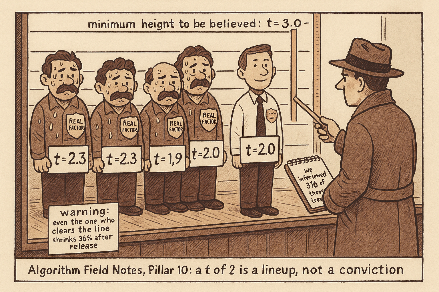
Test 316 factors at a t of 2 and about 16 are pure luck. The factor zoo is a multiple-testing failure: raise the bar to t above 3, expect a 36% out-of-sample haircut, but don't prune to five.

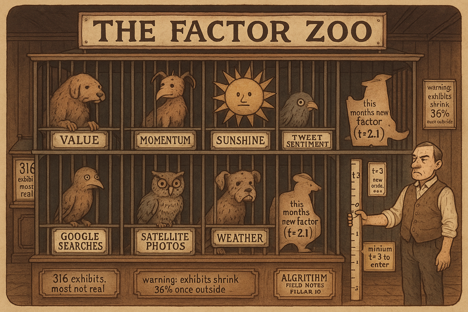
The old articles built the machine that grades a factor. Sort the cross-section, run the GRS test, run Fama-MacBeth, and out pops a t-stat. Every one of those tools treats your factor as if it were the only hypothesis you ever tried. It never is. The profession has run that machine on hundreds of candidate signals, kept the winners, and buried the losers in unpublished drawers, and the survivors get reported with a t-stat of 2 as if it meant something. It does not. A t of 2 is a 5% false-positive bar, and if you test three hundred dead signals, roughly fifteen of them clear that bar by luck alone.

That pile of survivors has a name: the factor zoo. Harvey, Liu, and Zhu cataloged more than three hundred published factors, and the number keeps climbing as researchers mine trading accounts, order books, social media, news text, satellite images, weather, and Google search volume for anything that correlates with next month's returns. Most of the zoo is noise that got published because nobody adjusted the significance bar for the search. This is the cross-sectional twin of the backtest-overfitting problem from the old articles "CSCV: A Direct Probability of Backtest Overfit" and "Permutation Tests for Indicator Significance." There the danger was one researcher sweeping parameters. Here it is a whole field sweeping signals.

The zoo is real and it is enormous

Look at where the candidate signals come from now. Trading account records, limit order book events, message-board sentiment, crowdsourced earnings forecasts, the text of 10-K filings, photographs in news articles, sunshine in the city where the exchange sits, and search-engine attention. Each data source spawns dozens of characteristics, each characteristic gets sorted into a long-short portfolio, and each portfolio gets a t-stat. Multiply it out and the count of tested signals runs into the thousands even if only three hundred reach print.

Quantity is the tell. When a field produces a new priced factor every few weeks for two decades, the base rate says most of them cannot be real, because real compensated risks are scarce and the market is not that inefficient in that many independent ways. The skeptic's default is that a freshly published anomaly is a false discovery until it survives a correction for how many signals were tried to find it.

Why one t-stat lies when you ran three hundred

Start with the arithmetic that breaks the naive t-stat. A single test at the 5% level has a 5% chance of a false positive when the factor is truly worthless. Run K independent such tests on worthless factors and the chance that at least one prints significant is not 5%, it climbs fast.

$$ \text{FWER} = \operatorname{prob}(\text{at least one false positive}) = 1 - (1-\alpha)^K $$

That is the family-wise error rate, the probability of making even one false discovery across the whole family of K tests, where alpha is the per-test level. Read it as one minus the probability that every single test correctly stays quiet. Work it for the zoo. With alpha of 0.05 and K equal to 316, one minus 0.95 to the power 316 is 0.99999991, indistinguishable from certainty. You are not at risk of a false factor, you are guaranteed a crowd of them. The expected count is even more concrete: if all 316 candidates were truly worthless, alpha times K is 0.05 times 316, about 16 factors clearing a t of 2 by pure luck. The zoo has a false-discovery floor baked in.

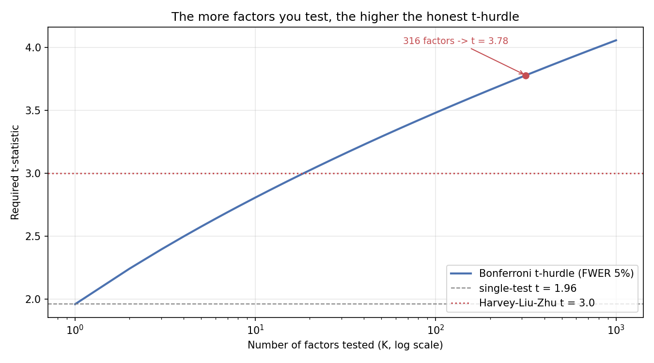
Curve showing the required t-statistic hurdle rising with the number of factors tested on a log scale, crossing t equals 3 near 20 factors and reaching 3.78 at 316 factors

The fix is to raise the bar as the search widens. The curve shows exactly how much. Test one factor and a t of 1.96 is fine. Test twenty and the honest hurdle is already past 3. Test the 316 of the published zoo and it sits near 3.8. The single-test t of 2 that fills asset-pricing papers is calibrated for a world where you tried one idea, and nobody tried one idea.

The error table: FWER, FDR, FDP

Multiple-testing control formalizes the bookkeeping. Sort every test into whether the factor is truly worthless or truly priced, and whether you rejected the null or not. Of K factors, K-zero are truly worthless and K-one are truly priced. You reject L of them, and those rejections split into T-one true discoveries and F-one false discoveries. Three different error rates target three different fears.

$$ \text{FWER}=\operatorname{prob}(F_1 \geq 1)\leq\alpha, \qquad \text{FDR}=\mathbb{E}\!\left[\frac{F_1}{L}\right]\leq\alpha, \qquad \text{FDP}=\operatorname{prob}\!\left(\frac{F_1}{L}\geq\gamma\right)\leq\alpha $$

The family-wise error rate caps the probability of even one false factor in the whole batch, which is brutally strict when K is large. The false discovery rate is gentler: it caps the expected fraction of your discoveries that are false, so if you announce 20 factors and accept an FDR of 5%, you tolerate about one of them being junk on average. The false discovery proportion caps the probability that the junk fraction exceeds some threshold gamma, a middle ground. Work the FDR: announce L equal to 20 factors at an FDR of 0.05 and you expect F-one near 1, so nineteen are likely real and one is likely noise, which is a very different promise from "each of these has a t of 2."

Two corrections: Bonferroni and Benjamini-Hochberg

The oldest correction is Bonferroni, and it controls the family-wise rate by brute force. Divide the significance level by the number of tests.

$$ \text{reject factor } i \text{ if } \; p_i \leq \frac{\alpha}{K} $$

Every factor must clear a per-test bar of alpha over K. With alpha of 0.05 and K of 316, the threshold is 0.05 divided by 316, which is 0.000158, and a two-sided p-value that small corresponds to a t-stat of about 3.8. Bonferroni is simple and safe and throws away real factors, because holding the probability of any false positive to 5% across hundreds of tests forces the bar so high that weak-but-genuine premia get rejected too.

Benjamini and Hochberg traded that severity for power. Instead of guarding against any false positive, they control the false discovery rate. Sort the p-values from smallest to largest, then walk down the list.

$$ \text{reject the } i \text{ smallest } p\text{-values, where } i \text{ is the largest index with } \; p_{(i)} \leq \frac{i}{K}\,\alpha $$

The threshold slides: the smallest p-value is judged against alpha over K, the second against two-alpha over K, and so on, so a factor does not have to clear the full Bonferroni bar if many other factors are also significant. It keeps more true discoveries while still capping the junk fraction. Harvey, Liu, and Zhu ran these corrections across the published zoo and landed on a practical hurdle: a factor needs a t-stat above about 3.0, not 2.0, before you should believe it. That single number retires a large slice of the literature, and it is the correction the old articles "CSCV: A Direct Probability of Backtest Overfit" and "Permutation Tests for Indicator Significance" were pointing at from the time-series side.

The 36% haircut: attenuation out of sample

Clearing the corrected bar in-sample is still not the finish line. Even factors that pass decay once you leave the sample they were discovered in. Harvey and Liu measured the drop at about 36% for U.S. stocks, and the deck's author reports a similar attenuation for the Chinese market. A factor with an in-sample premium of 6% a year is a 3.8% factor once real trading meets it, before costs.

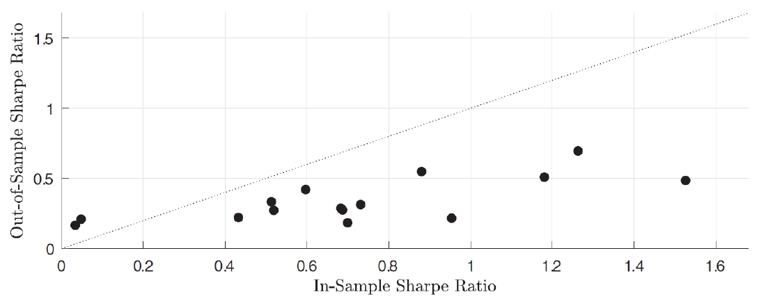
Scatter of in-sample against out-of-sample annualized Sharpe ratios for fifteen anomaly strategies, with every point sitting below the 45-degree line

The scatter makes the haircut visual. Fifteen anomalies, in-sample Sharpe on one axis and out-of-sample Sharpe on the other, and every point sits below the 45-degree line where the two would match. Nothing lands above it. The ranking survives, better in-sample strategies tend to be better out of sample, but the level shrinks across the board. That gap is the combined bill for the multiple testing that found the factor and the crowding that arrives once it is public, the same alpha-decay-is-competition theme from earlier pillars, now measured on the cross-section.

The illusion of sparsity

The obvious reaction is to prune hard: keep three or four factors and throw the zoo out. The data says that overcorrects. Giannone and coauthors called it the illusion of sparsity, and Kozak, Nagel, and Santosh showed it directly for the cross-section of returns. When you build the pricing kernel that actually maximizes out-of-sample Sharpe, it does not load on a handful of characteristics. It spreads weight across almost all of them.

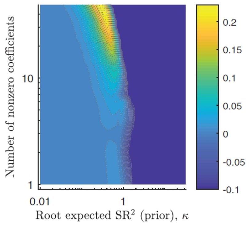
Contour plot of out-of-sample performance against prior strength on one axis and number of nonzero coefficients on the other, with the bright high-performance region requiring many nonzero coefficients

The bright region, where out-of-sample predictability peaks, sits at a large number of nonzero coefficients paired with a moderate prior. Shrink to a sparse handful of factors and you slide off the good region into the dark. So the reckoning cuts both ways. Most individual published factors are false, which argues for a higher bar. But the true pricing kernel is not sparse, which argues against compressing everything into five factors. The resolution is not a t-stat lottery and not a five-factor dogma. It is heavy shrinkage toward the whole cross-section under an economic prior, and the prior comes from theory: Kozak, Nagel, and Santosh argue that any factor with a high premium must also be a major source of comovement, because otherwise it would offer a near-arbitrage Sharpe ratio that cannot survive. Return has to be tied to risk structure, or it is a ghost.

Where this connects

The factor zoo is backtest overfitting scaled from one desk to an entire profession. The old article "CSCV: A Direct Probability of Backtest Overfit" measures how badly a single parameter search will disappoint out of sample; the multiple-testing correction here measures how badly a signal search across thousands of candidates will. The old article "Permutation Tests for Indicator Significance" builds a null distribution from the data so one indicator's p-value is honest; the corrections in this article fix the threshold once you admit you computed that p-value hundreds of times. Same disease, two scales.

The next step is that the tightest bar is not the right bar. Pushing the hurdle to a t of 3 kills false factors but also throws away real, diversifying ones, and the out-of-sample information ratio of a factor book can peak well below the strictest cutoff. Where that optimum sits, and why the selection-versus-diversification tradeoff means the academy's significance bar and the practitioner's diversification bar point in opposite directions, is the subject of the FDR-curve article to come.

KEY POINTS

The factor zoo is the pile of more than three hundred published factors mined from trading accounts, order books, text, images, weather, and search data. Most are false discoveries because the significance bar was never adjusted for how many signals were tried.
A t-stat of 2 is a single-test 5% bar. Test K worthless factors and the chance of at least one false positive is one minus 0.95 to the power K, which for the 316-factor zoo is essentially certain, with about 16 factors expected to clear t of 2 by luck.
Multiple-testing control targets three different errors: the family-wise error rate caps the probability of any false factor, the false discovery rate caps the expected fraction of discoveries that are false, and the false discovery proportion caps the probability that fraction exceeds a threshold.
Bonferroni divides the significance level by K and needs a t near 3.8 for 316 tests, which is safe but throws away real factors. Benjamini-Hochberg controls the false discovery rate with a sliding threshold, keeping more true discoveries. Harvey, Liu, and Zhu land on a practical hurdle of t above 3.0, not 2.0.
Survivors still decay: Harvey and Liu found about 36% out-of-sample attenuation for U.S. stocks, similar in China. A 6% in-sample premium becomes about 3.8% before costs, and every one of fifteen anomalies had a lower out-of-sample than in-sample Sharpe.
The illusion of sparsity: you cannot fix the zoo by pruning to a handful of factors, because the pricing kernel that maximizes out-of-sample Sharpe loads on almost all characteristics. The fix is heavy shrinkage toward the whole cross-section under an economic prior, not a five-factor dogma.
The economic prior: a high-premium factor must also drive comovement, or it implies a near-arbitrage Sharpe ratio that will not survive. Return tied to risk structure is real; return untethered from it is a ghost.

References

- ... and the Cross-Section of Expected Returns (Harvey, Liu, and Zhu, 2016)
- Presidential Address: The Scientific Outlook in Financial Economics (Harvey, 2017)
- Lucky Factors (Harvey and Liu, 2021)
- Controlling the False Discovery Rate: A Practical and Powerful Approach to Multiple Testing (Benjamini and Hochberg, 1995)
- Shrinking the Cross-Section (Kozak, Nagel, and Santosh, 2020)
- Interpreting Factor Models (Kozak, Nagel, and Santosh, 2018)
- Economic Predictions with Big Data: The Illusion of Sparsity (Giannone, Lenza, and Primiceri, 2021)
- A Forward Looking View of Factor Investing, DDA3600: Factor Investing (Chuan Shi, 2024)
A note on AI. The ideas, research, analysis, and conclusions in this article are my own. I use AI tools to help with editing and wordsmithing, because English is not my first language, and I am not shy about that. AI-generated ideas and AI-assisted writing are not the same thing: the first is empty slop from a generic prompt, the second is a tool for communicating years of real research more clearly. Judge the work by its substance, not by whether software helped polish the prose.