10.20 A Trend Factor for the Crypto Cross-Section (and Its Overfit Tell)

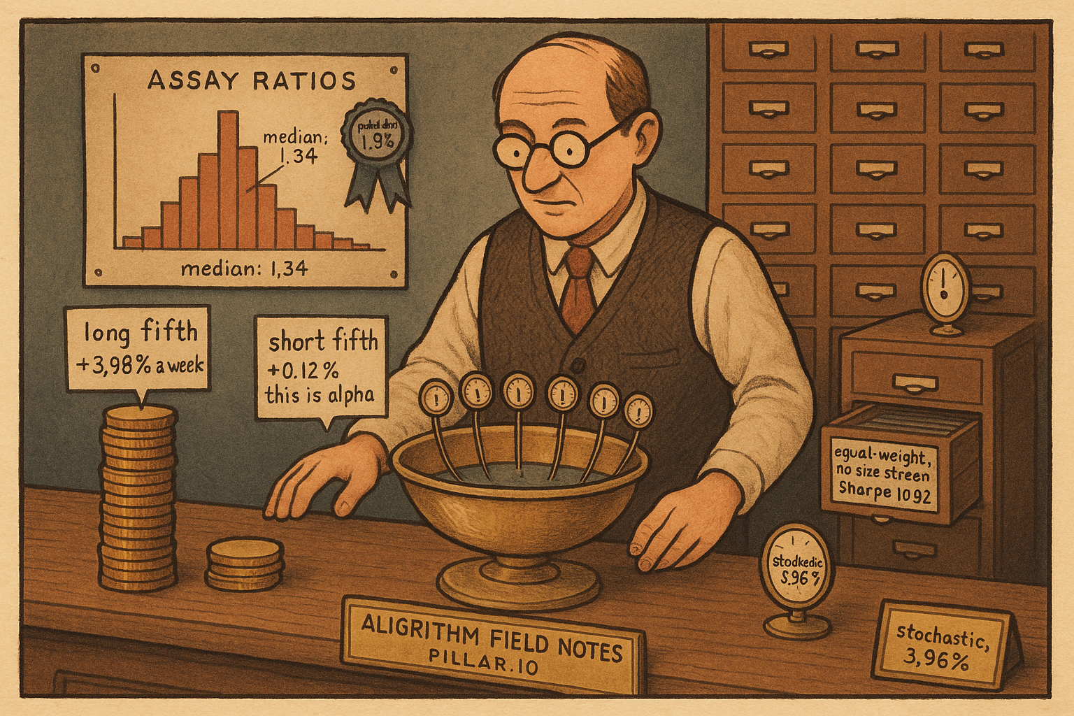
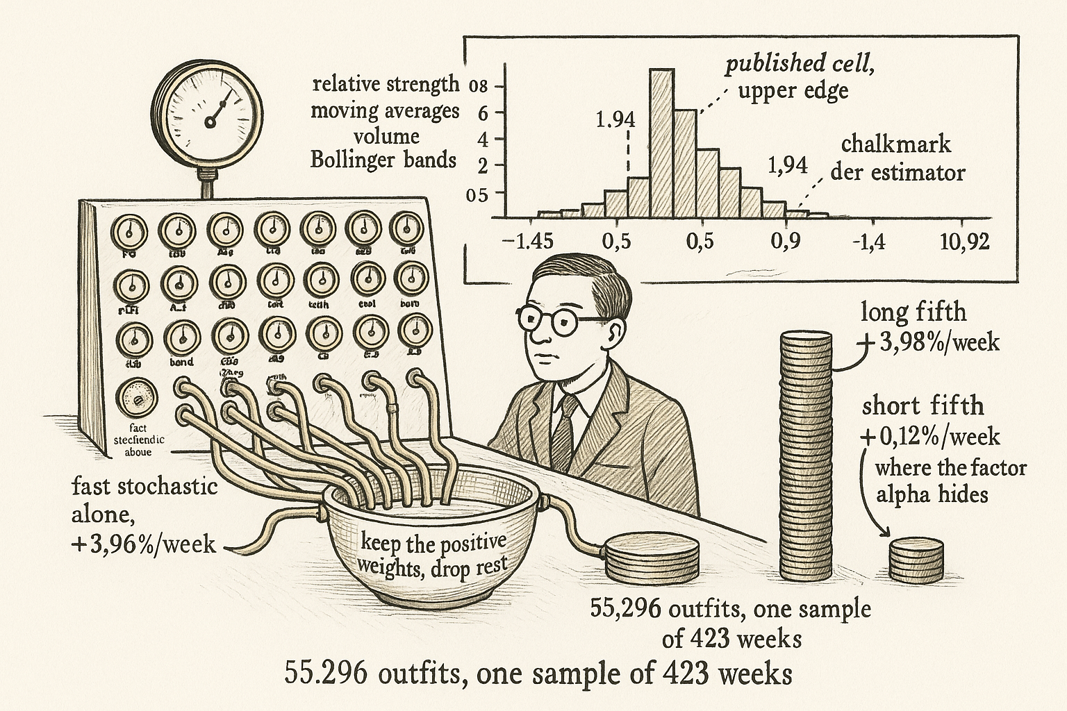
Fieberg, Liedtke, Poddig, Walker, and Zaremba build a weekly score from 28 technical indicators, buy the value-weighted top fifth of coins, and short the bottom fifth. From April 2015 to May 2022 that hedge earns 3.87% a week, t-statistic 5.19, annualized Sharpe ratio 1.94. They then rebuild the same trade under 55,296 research designs. The published Sharpe sits at the upper edge of that pile. The median Sharpe of the estimator they recommend is 1.34, and the cell that equal-weights coins with the million-dollar size screen turned off prints 10.92. The ranking is a pattern in this sample. The 1.94 is the friendly cell.

What this actually is

A coin book has no earnings to sort on. Market cap is a supply figure the issuer can mint, and the tape you can recompute is price and volume. The desk question is whether a stack of chart readings, combined by a shrinkage regression, ranks next week's returns well enough to pay for replacing about two-thirds of the weights every week.

Each week the method turns 28 chart readings into separate forecasts of next week's return, throws out the forecasts with the wrong sign, and averages the rest into one score. They call that average CTREND. The trade is a value-weighted long-short of the top and bottom fifths, held for one week.

Picture a clerk who refuses to trust one dial. He writes down a relative-strength reading, a stochastic, seven moving averages, a volume oscillator, and a Bollinger band for every coin. He checks, over the last 52 weeks, which dials pointed the same way as the following week's return, throws out the dials that pointed the wrong way, and averages the survivors. The average is the score. Top fifth against bottom fifth is the trade.

If that score survived a one-day delay, a validation slice, and a multiple-testing haircut, you would swap a 2-to-4-week momentum sort for it and you would drop momentum out of a crypto factor model. If 1.94 is the upper edge of a 55,296-cell grid on one sample of 423 weeks, you would underwrite the median cell, and you would put the t-statistic of 5.19 through the old article "The Factor Zoo and the Multiple-Testing Reckoning" before you sized a book on it.

Twenty-eight dials, then an average

This section settles whether the combiner beats the best single oscillator, or lands next to it.

CoinMarketCap, weekly, April 2015 through May 2022, 423 weeks. A coin-week needs a close, a dollar volume, and a market cap. They delete the ten daily prints in which some coin's cap exceeds Bitcoin's, require a cap of at least 1 million dollars, and truncate returns at the 0.5 and 99.5 percentiles. Table 1 counts 3,245 unique coins. The prose says 3,244. One coin, unexplained. The table stands.

The 28 inputs sit in four groups, at fixed horizons taken from the technical-analysis literature, which is how the authors keep the window lengths out of the search. Oscillators: the 14-day relative strength index (average up-move divided by average down-move), a stochastic of that index, the fast and slow stochastics (where the close sits in the 14-day high-low range, and a 3-day average of that), and the commodity channel index. Moving averages: simple averages at 3, 5, 10, 20, 50, 100, and 200 days, each divided by the week's close so a high-priced coin does not dominate, plus the gap between a 12-day and a 26-day exponential average as a percent of the fast one, and that gap minus its 9-day signal. Volume: the same seven lengths of dollar volume divided by current volume, the volume versions of that gap and its signal, and Chaikin money flow. Volatility: Bollinger lower, middle, and upper bands divided by price, and the bandwidth.

Every indicator is replaced by its cross-sectional rank, mapped into the interval from -0.5 to +0.5, so the lowest coin that week sits at -0.5 and the highest at +0.5. The paper states the interval and does not print the interpolation. Regressions are fit by value-weighted least squares, weights proportional to market cap, so a microcap's residual barely moves a slope. The combiner is imported from the equity trend factor of Han, Zhou, and Zhu and from the cross-sectional elastic net of Han, He, Rapach, and Zhou. It was built for stocks. Crypto is the new tape.

Each week, for each indicator, they run a cross-sectional regression of this week's return on last week's rank. The intercept and the slope that enter the forecast are the arithmetic means of those weekly estimates over a rolling 52-week window. The first score therefore does not exist in April 2015. The table captions still date the study from April 2015.

$$ \hat{r}^{j}_{i,t+1} = \bar{\alpha}_{j,t} + \bar{\beta}_{j,t}\, z_{i,j,t} $$

Read it as: the forecast of coin i's next-week return from indicator j equals the 52-week-averaged intercept, in percent per week, plus the averaged slope times the coin's current rank. The rank is a pure number between -0.5 and +0.5. The forecast is in percent per week. Worked illustration, not a coefficient from the paper. An averaged intercept of 0.80 and an averaged slope of 5.0 send a coin at rank +0.30 to 0.80 + 5.0 times 0.30, which is 2.30 percent. The same dial at rank -0.30 sends it to 0.80 minus 1.50, which is -0.70 percent.

They repeat that for all 28 indicators, then regress realized return on the 28 forecasts with an elastic net. The penalty is a half-and-half mix of the sum of absolute weights and the sum of squared weights, and the penalty strength is chosen by the corrected Akaike criterion. A forecast whose fitted weight is positive stays. A forecast whose weight hits zero or goes negative is dropped. The score is the equal-weighted average of the survivors. Their equation (11) is this average. The printed notation uses one symbol for the index, the set, and the count. The denominator is the number of forecasts with a positive weight.

$$ \mathrm{CTREND}_{i,t+1} = \frac{1}{|J^{+}|} \sum_{j \in J^{+}} \hat{r}^{j}_{i,t+1}, \qquad J^{+} = \{ j : \theta_{j} > 0 \} $$

Read it as: CTREND for coin i next week is the arithmetic mean of the univariate forecasts whose elastic-net weight theta is positive. Each forecast is in percent per week, and so is the mean. Worked continuation of the illustration. The coin's first forecast is 2.30 percent and a second survivor is 1.26 percent. The score is (2.30 + 1.26) / 2 = 1.78 percent. Dividing by 28 instead of by 2 would print 0.13 percent and would throw away the selection step. A third forecast with a negative weight does not enter, and it is not flipped into a reversal signal. In this sample that restriction fits the tape: the relative strength index, a textbook reversal tool, has a high-minus-low return of +3.52% a week (t-statistic 5.41). Coins the oscillator calls overbought keep rising.

The ingredients already pay. The fast stochastic's high-minus-low earns 3.96% a week (t-statistic 5.73), and its alpha against the Liu, Tsyvinski, and Wu three-factor model is 2.56% (t-statistic 4.13). The combined score earns 3.87% (t-statistic 5.19) and a three-factor alpha of 2.62% (t-statistic 4.22). On raw return the stochastic leads by 0.09 points. On three-factor alpha the score leads by 0.06 points, six basis points a week. The authors' appendix ranks the middle Bollinger band, the commodity channel index, and the convergence/divergence as the heaviest inputs. A blend can load on several dials and still land its portfolio next to the strongest dial.

Moving-average signs run the other way, and the reason is the scaling. They divide the average by price, so a high reading means the average sits above the price and the coin has been falling. The 5-day average's high-minus-low is -2.90% a week (t-statistic -3.35). The continuation trade is the low reading, price above its average. A negative high-minus-low column is the trend, with the sign flipped by the scaling.

The 3.87% is the long book

This section settles who pays the 3.87%, the coins you buy or the coins you short.

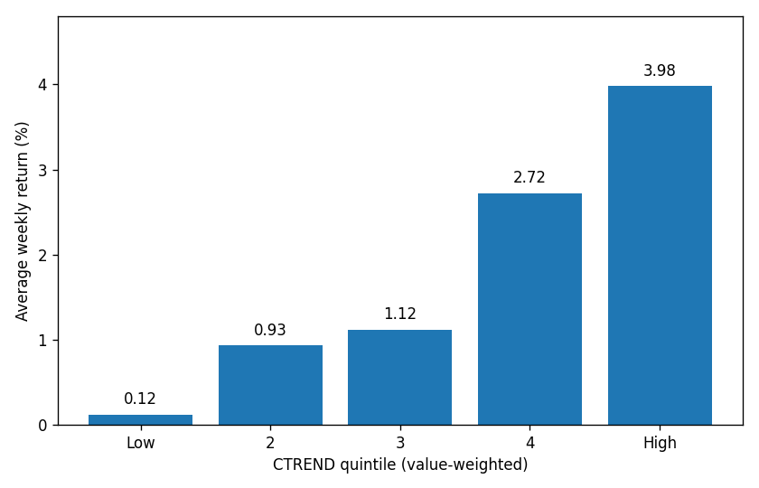
Value-weighted quintiles, rebalanced every week. Average weekly returns, in percent: low 0.12 (t-statistic 0.16), then 0.93, 1.12, 2.72, and high 3.98 (t-statistic 4.80). The high-minus-low row prints 3.87. The two extremes differ by 3.86, and the extra hundredth is rounding. The step from the third quintile to the fourth is 1.60 points. The step from the second to the third is 0.19. The spread lives in the tails, and the bottom fifth earns about zero.

$$ SR = \frac{\bar{r}}{s} \sqrt{52} $$

Read it as: the annualized Sharpe ratio is the weekly mean return divided by the weekly standard deviation, times the square root of 52. Both the mean and the standard deviation are in percent per week, so the ratio is a pure number. The square root of 52 is the right scale when the weeks are uncorrelated. Worked with Table 3's high-minus-low row. Mean 3.87, standard deviation 14.34. The weekly ratio is 3.87 / 14.34 = 0.2699. Times the square root of 52, which is 7.211, that is 1.946. The table prints 1.94. The third digit moves with rounding of the two inputs. The other five quintile Sharpes in the same table recover from their printed means and standard deviations without that gap. Multiply 3.87 by 52 and you get 201 percentage points, arithmetic, before a week with a 14.34% standard deviation has been allowed to hurt the book. The 1.94 is the number that includes the volatility.

The hedge's market beta is 0.03 (t-statistic 0.50) and its size beta is -0.08 (t-statistic -1.79). Its momentum beta is 0.79 (t-statistic 14.88). Alpha against the one-factor crypto market model is 3.80% a week (t-statistic 5.03). Alpha against the three-factor model is 2.62% (t-statistic 4.22).

Split that 2.62. The high quintile's three-factor alpha is 1.10% with a t-statistic of 1.94, which misses the 5% line the authors use for boldface. The low quintile's alpha is -1.51% (t-statistic -3.23). Taking 1.10 minus a negative 1.51 gives 2.61, against the printed 2.62. The raw return is the long book: 3.98% minus a bottom fifth that earns 0.12%. The alpha the factor model cares about is the short book failing to earn its premium. The bottom fifth is the smaller one. Average market cap is 135 million dollars there and 1,182 million in the top fifth. Average cumulative return over the prior three weeks is -21.63% in the bottom fifth and +62.74% in the top fifth. That gap is why the momentum beta is 0.79. The top fifth itself carries a momentum beta of 0.52, and the bottom fifth carries -0.27. The difference is the hedge's 0.79.

A double sort leaves a long-short between 1.42% and 3.10% a week after a momentum control at one to four weeks. The Fama-MacBeth slope, a cross-sectional coefficient fit separately each week and then averaged, stays between 2.00 and 2.94 with those controls in, and prints 2.62 (Newey-West t-statistic 3.93; the standard errors allow for autocorrelation) when every control enters at once. The univariate slope is 2.36 (t-statistic 5.00). If the score is already in percent per week, 2.36 says one point of predicted return lines up with 2.36 points of realized return. Averaging noisy forecasts shrinks the score's cross-sectional spread, and a second-stage slope above one is what that shrinkage looks like. The paper never prints the spread, so the 2.36 stays a slope per unit of the score. The control that bites is the Amihud illiquidity ratio, absolute weekly return divided by dollar volume. After that double sort the three-factor alpha is 0.62% and clears the 10% line.

One sample, 55,296 outfits

This section settles what "it works in 55,296 specifications" is worth.

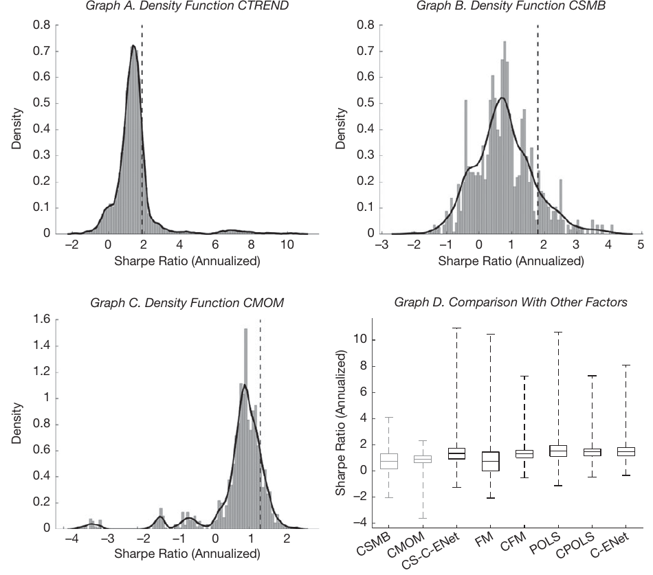
The grid multiplies switches: how you treat outliers, whether stablecoins stay in, the cap screen, a one-dollar price screen, rolling versus expanding windows, 26 to 104 weeks of estimation, a lag of zero or one day, quintiles versus tertiles, value weights versus equal weights, and whether the volume indicators are included. Six estimators sit on that common grid. The figure caption's comparison uses 6,144 designs. The text says 55,296 combinations. Those two numbers divide evenly, 55,296 / 6,144 = 9. Panel C of their design table adds a validation switch and a forecast-weight switch that are filled in only for the elastic-net column. Five plain estimators plus four elastic-net variants is nine. The paper does not write the multiplication. The product is the grid, and every cell is the same 423 weeks.

Graph A is the density of Sharpe ratios across all 55,296 cells. The dashed line is the published specification, and the authors place it at the upper edge. Most of the mass lies between 0.5 and 2.5. For the elastic-net estimator alone the Sharpe runs from -1.45 to 10.92, and the median is 1.34. The 10.92 is the corner that equal-weights coins and turns the million-dollar cap screen off. Using Lo's test, which judges whether a Sharpe ratio is positive once the standard error allows for autocorrelation, 79% of all combinations clear 5%. The size factor clears that bar in 56% of its designs (median Sharpe 0.94, maximum 4.60). Momentum clears it in 49% (median 0.83, maximum 2.30, minimum -4.47).

Read the entries in their Table 6 as conditional medians. Each row holds one switch fixed and takes the median over everything else. Holding the elastic net, a few switches move that median by enough to matter. With no validation sample the median Sharpe is 1.47. When the most recent 12 weeks are used only to decide which forecasts survive, it falls to 1.19. A zero implementation lag prints 1.46. A one-day lag, the version you can run after the close, prints 1.24. A price screen at zero prints 1.64. A screen at one dollar prints 1.13. Dropping every volume indicator moves the median from 1.30 to 1.39, so exchange wash volume is not where this Sharpe lives.

The plain multivariate regression, the original Han, Zhou, and Zhu estimator, is the wide, low box in the comparison panel. Averaging the univariate forecasts and then keeping the positive weights is what tightens the distribution. That is a methods result, and it is the part worth taking to another market. The level of the crypto Sharpe is a separate claim, and it moves when you delay the trade by a day or when you stop selecting indicators on the weeks you score.

A t-statistic of 5.19 belongs to one cell. The cells share one sample, and a 79% hit rate is what a small perturbation of a positive sample looks like. The old article "The Factor Zoo and the Multiple-Testing Reckoning" is the tax on publishing the cell near the top. The number their own grid supports is the elastic-net median, 1.34, and the validation-sample median, 1.19. Both beat momentum's median of 0.83. Quote 1.34, or 1.19 when the surviving indicators are chosen on a held-out 12 weeks.

It prices the strategies it was built from

This section settles whether swapping momentum for this score prices the cross-section, or prices the indicators that went into the score.

They form tangency portfolios out of sample. Weights are estimated on the prior 52 weeks, the book is rescaled to a weekly volatility of 10%, and the weight is the usual mean-variance one: the inverse covariance matrix times the mean vector, normalized to sum to one. Adding the trend factor to the three-factor tangency portfolio produces an alpha of 2.77% a week (Newey-West t-statistic 3.80). Adding momentum to a model that already has the market, size, and the trend factor produces 0.37% (t-statistic 1.02). On this test, momentum is the factor that does not expand the frontier.

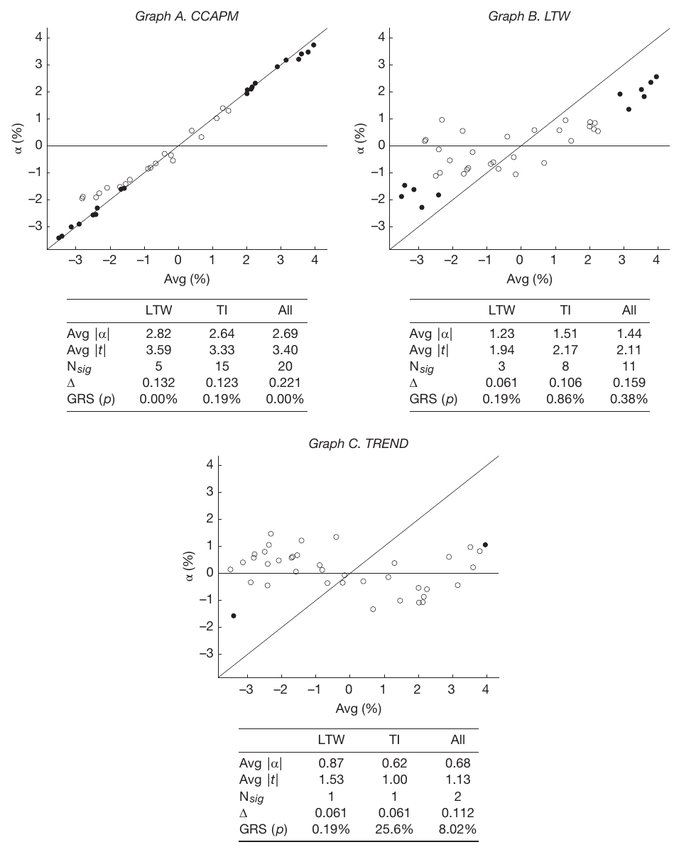
The scatter compares each anomaly portfolio's average return with the alpha a model leaves behind. On the 45-degree line, alpha equals the average return. A cloud around the horizontal axis means the alphas are near zero. The Gibbons, Ross, and Shanken statistic tests the joint claim that every alpha is zero. The one-factor market model leaves an average absolute alpha of 2.69%, 20 portfolios still individually significant, joint-test p-value 0.00%. The three-factor model leaves 1.44%, 11 significant, p-value 0.38%. The model that swaps momentum for the trend factor leaves 0.68%, 2 significant, p-value 8.02%.

Split the pooled row, because that is where the win sits. On the technical-indicator portfolios the p-value goes from 0.86% under the three-factor model to 25.6% under the trend model, and the count of significant alphas goes from 8 to 1. On the Liu-Tsyvinski-Wu anomalies, which include size and the momentum horizons, the p-value is 0.19% under both models, and the weighted pricing error stays at 0.061. The pooled pricing error falls from 0.159 to 0.112 because the technical-indicator error falls from 0.106 to 0.061. A score blended from those indicators should price those indicators. The paper also says the trend model explains the momentum sorts, and names the two leftovers: the size quintile, and the fast stochastic, with a t-statistic of 1.98. The size miss has a mechanical piece they state themselves. Their size factor is a tercile sort, and the quintile sort they are trying to price has a wider spread. No model they try passes the test on that anomaly set.

Large coins and a 68% weekly turnover

This section settles what is left once you refuse the microcaps and you pay to trade.

Inside the largest half of coins by cap, the hedge earns 3.84% a week (t-statistic 5.00). Inside the largest tenth, 2.51% (t-statistic 3.01), with a three-factor alpha of 2.02% (t-statistic 3.18). Inside the most liquid tenth by the Amihud ratio, 2.20% (t-statistic 2.76), alpha 1.97% (t-statistic 3.18). The largest 100 coins earn 3.39% (t-statistic 4.49) in the size table and 3.40% (t-statistic 4.48) in the cost table. A hundredth. The spread survives after the small half is gone. It is largest in the liquid half, at 4.36% a week (t-statistic 5.62). The top tenth is where about a third of the full-sample 3.87% disappears.

$$ r^{\mathrm{net}} = r^{\mathrm{gross}} - \left( c_{L} \cdot 2 \cdot TO_{L} + c_{S} \cdot 2 \cdot TO_{S} \right) $$

Read it as: net and gross returns are in percent per week. Turnover is the fraction of a leg they print, and the 2 turns that half-sum into the fraction of weight traded. The cost rates are in percent per unit of weight traded, so a 30 basis-point long leg enters as 0.30. Worked with the printed turnovers, 62.84% on the long leg and 74.09% on the short leg, at 30 basis points long and 40 short. The long-leg cost is 0.30 times 2 times 0.6284, which is 0.377. The short-leg cost is 0.40 times 2 times 0.7409, which is 0.593. The sum is 0.970 percentage points. Subtract from 3.87 and you get 2.90, the net return they print (t-statistic 3.89). At 0.50 long and 0.60 short the cost is 0.50 times 1.2568 plus 0.60 times 1.4818, which is 1.517, and 3.87 minus 1.517 is 2.35 (t-statistic 3.16).

Their net-return equation writes the cost on the raw change in weight. The turnover equation above it grows last week's weight by one plus the coin's return before taking the difference. The printed net returns reconcile with twice the printed turnover, so the card uses the turnover equation. A flat cost rate that zeros the 3.87% mean divides 3.87 by the total weight traded, 2 times (0.6284 + 0.7409) = 2.7386. Then 3.87 / 2.7386 = 1.413%, and they print a breakeven of 1.41%. The rate that pushes the t-statistic through 5% is 0.88%. On the largest 100 coins the gross mean is 3.40%, turnover is 68.21%, the 30/40 basis-point net is 2.45%, and the breakeven flat rate is 1.25%.

Holding for two weeks instead of one cuts the average weekly return by what they call 1.5 percentage points, to 2.34%. Subtracting 1.5 from 3.87 gives 2.37, not 2.34, so the "1.5" is rounded and 2.34 is the number in the supplement. They say the mean stays past the 5% line out to a four-week hold. That table is in the supplement.

The hedge replaces 68.46% of its weights each week. The old article "Percentile-Rank Momentum With Hysteresis: Low-Churn Signals" is the relevant patch: a band that keeps a coin in the book until the rank crosses out of the quintile. The four-week result says the mean is still past the 5% line at a one-month hold. The paper does not test the band. A different path summary sits in the old article "Price-Path Convexity: A New Cross-Sectional Anomaly (−45bp per σ)", which prices one functional of the equity path at -45 basis points per standard deviation. This score prices a bundle of 28 functionals of the crypto path. Leave the equity figure in that article.

Own the long fifth of large coins if you want the raw return and you can live with that leg's momentum beta of 0.52. Leave the 2.62% three-factor alpha on the hedge: 1.10 points of it sit on the long leg, t-statistic 1.94, and the rest is the short. Underwrite a Sharpe nearer 1.2 than 1.94 once the design includes a one-day lag and a validation slice, because that is where their own medians sit. The 68% weekly replacement against a 141 basis-point breakeven is a wide gate, measured on CoinMarketCap from 2015 to 2022, stablecoins out, returns already truncated at half a percent.

KEY POINTS

• CTREND averages the univariate 52-week Fama-MacBeth forecasts, among 28 ranked technicals, that keep a positive elastic-net weight. The value-weighted high-minus-low quintile earns 3.87% a week (t-statistic 5.19), weekly standard deviation 14.34%, printed Sharpe 1.94. The printed mean and standard deviation annualize to 1.946.
• The raw return is the long fifth, at 3.98%. The short fifth earns 0.12%. The three-factor alpha of 2.62% is mostly the short leg's alpha of -1.51%. The long leg's alpha is 1.10%, t-statistic 1.94. Momentum beta of the hedge is 0.79.
• The fast stochastic alone earns 3.96% a week and a three-factor alpha of 2.56%. The combiner adds six basis points of weekly alpha. Relative strength continues in this sample (+3.52% high-minus-low), the opposite of the textbook reversal reading.
• Across the elastic-net designs the Sharpe runs from -1.45 to 10.92, median 1.34. The published 1.94 sits at the upper edge of the 55,296-cell density. A 12-week validation slice drops the conditional median from 1.47 to 1.19. A one-day implementation lag drops it from 1.46 to 1.24. The 10.92 cell equal-weights coins and drops the million-dollar cap screen. 55,296 / 6,144 = 9, a product of switches on one sample.
• Swapping momentum for CTREND cuts average absolute anomaly alpha from 1.44% to 0.68% and lifts the Gibbons-Ross-Shanken p-value from 0.38% to 8.02%. The pricing-error drop lives in the technical-indicator portfolios. The Liu-Tsyvinski-Wu anomaly set still rejects, p-value 0.19%, with the weighted pricing error unchanged at 0.061.
• The spread survives in the largest tenth (2.51%) and the most liquid tenth (2.20%). Weekly turnover is 68.46%. At 30 basis points long and 40 short the net is 2.90%. The flat breakeven rate is 1.41%. A two-week hold prints 2.34% a week in the supplement; their "drop of 1.5 points" from 3.87 lands on 2.37, so the 1.5 is rounded.

References

• Han, He, Rapach, and Zhou (2024). Cross-Sectional Expected Returns: New Fama-MacBeth Regressions in the Era of Machine Learning
• Han, Zhou, and Zhu (2016). A Trend Factor: Any Economic Gains from Using Information over Investment Horizons?
• Liu, Tsyvinski, and Wu (2022). Common Risk Factors in Cryptocurrency
• Lo (2002). The Statistics of Sharpe Ratios
• Menkveld et al. (2024). Nonstandard Errors
• Fieberg, Liedtke, Poddig, Walker, and Zaremba (2025). A Trend Factor for the Cross Section of Cryptocurrency Returns

A note on AI. The ideas, research, analysis, and conclusions in this article are my own. I use AI tools to help with editing and wordsmithing, because English is not my first language, and I am not shy about that. AI-generated ideas and AI-assisted writing are not the same thing: the first is empty slop from a generic prompt, the second is a tool for communicating years of real research more clearly. Judge the work by its substance, not by whether software helped polish the prose.