10.14 Price-Path Convexity: A New Cross-Sectional Anomaly (−45bp per σ)

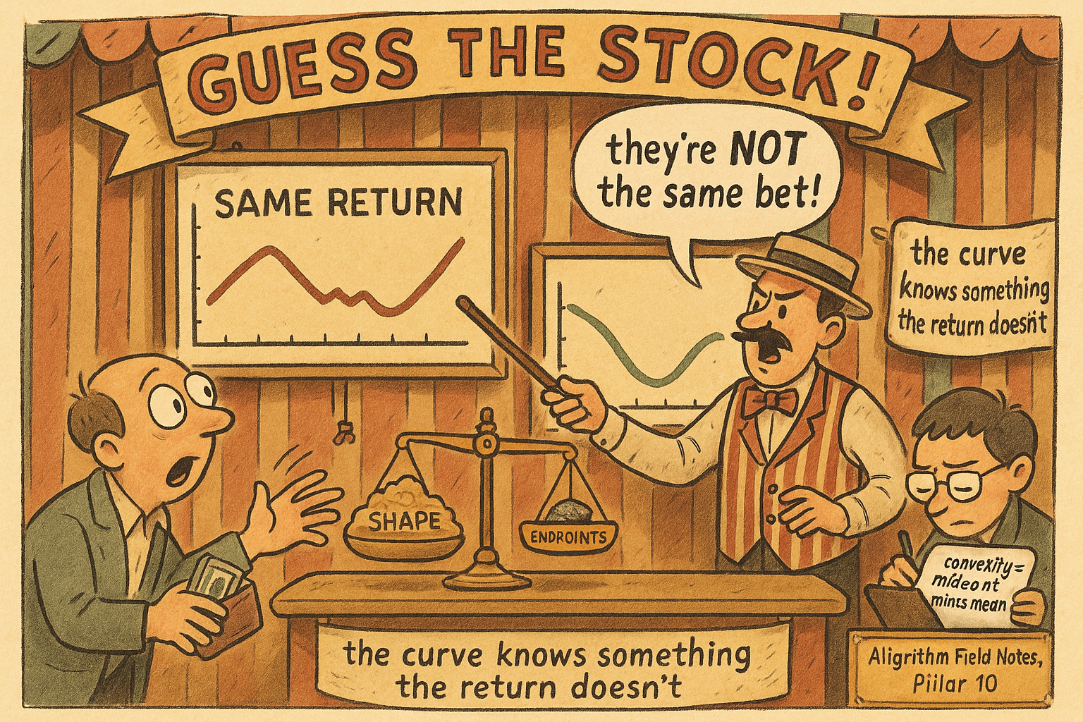
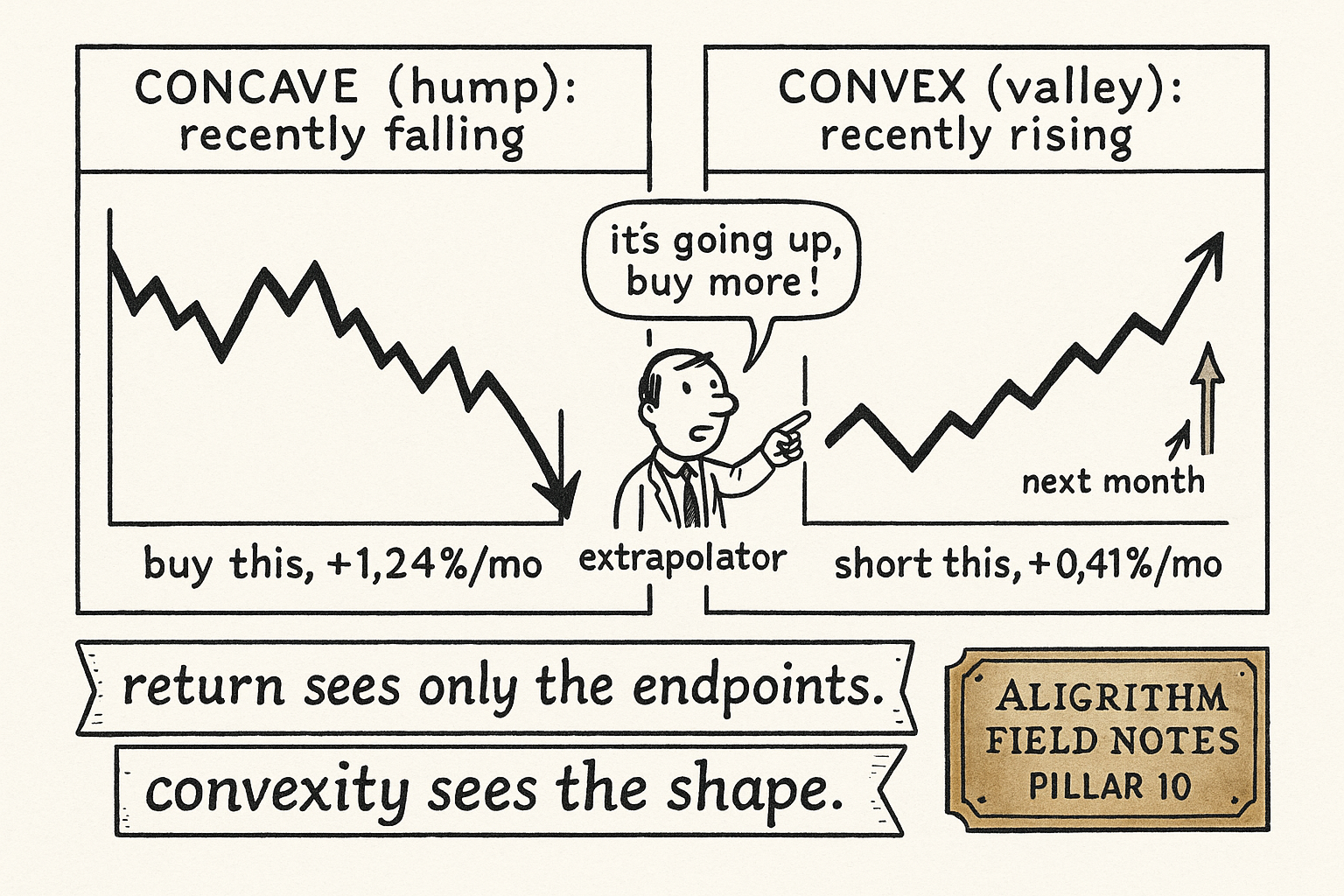
Take two stocks that both end the month flat. The first bled lower for two weeks, then clawed all the way back. The second ran up for two weeks, then gave it all back. Same start, same finish, same zero return. Sort every stock in the market by past return and these two land in the identical bucket, because return only sees the endpoints. Gulen and Woeppel show that the shape between the endpoints predicts next month, and it predicts it hard: the stock that ended by rising underperforms the stock that ended by falling by about 0.84% a month, and no standard factor touches the spread.

The old article "Wave Velocity and Acceleration: Reading When the Market Runs Out of Gas" argued that the second derivative of a price path carries an early read the level and slope miss. This is the cross-sectional version of that claim, tested on sixty years of the entire U.S. market instead of one instrument's sine fit. Return is the first derivative. Convexity, the curvature of the path, is a scaled cousin of the second derivative, and it prices the cross-section on its own.

What convexity measures, and how to compute it

Convexity compares two summaries of the same price path. Take the midpoint of the first and last closing price of the month. Subtract the average of every daily close in the month. Divide by the midpoint to standardize across price levels. That difference is the whole variable.

$$ \text{Convexity}_{it} = \frac{\dfrac{P_{1t} + P_{N_{it}}}{2} - \dfrac{1}{N_{it}}\sum_{k=1}^{N_{it}} P_{kt}}{\dfrac{P_{1t} + P_{N_{it}}}{2}} $$

Read it as midpoint of the endpoints, minus mean of the closes, over the midpoint. P-one is the first close of the month, P-N is the last close, and the middle sum is the average of all the closes in between. When the average of the closes sits below the midpoint of the endpoints, the path sagged in the middle and recovered, so convexity is positive and the path is convex, a valley. When the average sits above the midpoint, the path bulged up in the middle and faded, so convexity is negative and the path is concave, a hump.

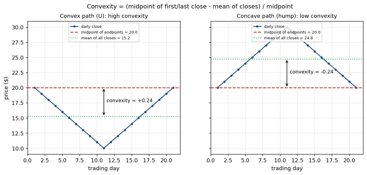
Work the paper's own example, in dollars. A stock opens the month at 20, drops 1 a day for ten days down to 10, then climbs 1 a day for ten days back to 20. First close and last close are both near 20, so the midpoint is 20. The average of all the closes is dragged down toward 15 by the trough. Midpoint minus mean is about 4.8, and 4.8 over 20 is roughly 0.24. That is a strongly convex path. Now steepen the front half: drop 1.50 a day for ten days to 5, then climb 1 a day, ending at 15. The average sinks further, the midpoint falls to 17.5, and convexity rises to about 0.42. A return measure would call both paths the same, since it only reads start and end. Convexity separates them because it weighs the whole trajectory.

The authors build it from price changes in dollars, not percentage returns, on purpose. Investors think about a stock in dollar terms as much as in percent terms (Shue and Townsend document the non-proportional thinking), and dollar changes track the path's actual dynamics better than a return that collapses to its endpoints.

The cross-sectional result: a monotone decline and a clean spread

Sort every NYSE, AMEX, and NASDAQ common stock into convexity quintiles at each month-end, form value-weighted portfolios, and hold one month. The pattern is monotone. The lowest-convexity quintile, the concave humps that just faded, earns 1.24% the next month. The highest-convexity quintile, the convex valleys that just rallied, earns 0.41%. Every step down in convexity rank buys you return.

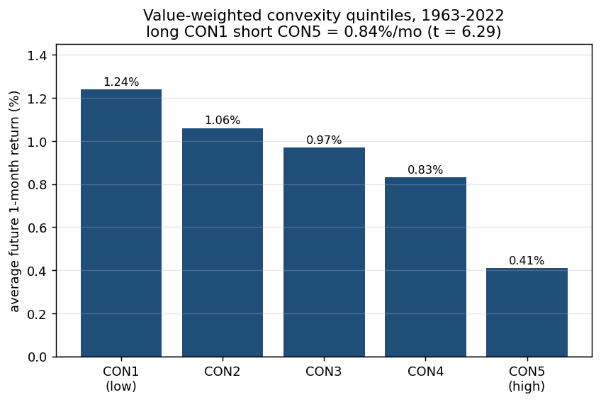
Buy the lowest quintile, short the highest, and the zero-investment spread is 0.84% a month with a t-stat of 6.29. That is a Sharpe of 0.23 monthly, which annualizes near 0.80. The old article "Portfolio Sorts From Scratch: Deciles, Monotonicity, and the Long-Short Spread" set the bar for trusting a sort: you want a monotone gradient across the buckets, not a lone extreme quintile carrying the whole spread. Convexity clears it, and it clears it at shorter horizons too, earning 0.64% per 10-day hold (t of 7.31) and 0.37% per 5-day hold (t of 4.94).

Then run the spread through the factor gauntlet. Regress the long-short return on CAPM, then the Fama-French three-factor model, then the five-factor model, then five-factor plus momentum, short-term reversal, long-term reversal, and liquidity. The alpha stays between 0.81% and 0.96% a month, every t-stat above 5.6. The factor models explain almost none of it. The spread's return also beats the best single factor in the sample (momentum) by 20 basis points, and its Sharpe runs more than half again above the second-best factor. During recessions the spread pays 1.55% a month. A premium that gets larger when the world is worse is the opposite of what a risk story predicts.

Is this just short-term reversal wearing a costume?

Short-term reversal is the oldest short-horizon anomaly in the book: last month's losers beat last month's winners next month. The old article "Reading Reversals from Autocorrelation" traced that effect to negative serial correlation at short lags. Convexity smells related, since a convex valley ends on an up-move and a concave hump ends on a down-move, and reversal would fade both. The obvious worry is that convexity is reversal with extra steps.

The double sort kills that worry. Sort independently on convexity and on lagged one-month return, then read the convexity spread inside each reversal bucket.

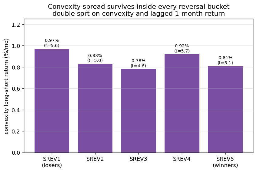
Inside every reversal quintile, from the biggest losers to the biggest winners, the convexity spread survives: 0.97%, 0.83%, 0.78%, 0.92%, and 0.81% a month, with t-stats from 4.60 to 5.69. Convexity predicts among stocks that all had the same past return. Run it the other way, hold convexity fixed and vary past return, and reversal mostly flattens out; in the lowest convexity quintile lagged return does not predict future return at all. So the curvature carries information the endpoints do not, which is the same lesson the old article "Legendre-Polynomial Trend and Trend Relative to Local Variation" pushed for a single series: a clean straight climb and a drunk stagger with the same net move are different trades, and you want a number that scores the shape, not just the displacement.

The 45 basis points that survive every control

Portfolio sorts can hide a correlated characteristic doing the real work. The fix is a Fama-MacBeth cross-sectional regression: each month, regress next month's return on this month's convexity plus a stack of controls, then average the monthly slopes and test whether the average slope is different from zero.

$$ R_{i,t+1} = \gamma_{0t} + \gamma_{1t}\,\text{Convexity}_{it} + \sum_{j} \gamma_{jt}\,\text{Control}_{j,it} + \varepsilon_{i,t+1} $$

R next month is stock i's return, the gammas are the slopes estimated fresh each month, and the reported number is the time-series average of the convexity slope with a t-stat corrected for autocorrelation. The controls are the usual suspects: size, book-to-market, profitability, asset growth, momentum, one-month return (that is short-term reversal), illiquidity, idiosyncratic volatility, skewness, and maximum daily return. With every control in the same regression, a one-standard-deviation increase in convexity is associated with a 45 basis point decline in the next month's return, at a robust t-stat of −11.15.

Put a number on it. Say the convexity distribution has a standard deviation of 0.05 in this month's cross-section. A stock one standard deviation above average convexity, so 0.05 more convex than the typical name, carries a predicted return roughly 0.45% lower next month than the average stock, holding size, momentum, reversal, and the rest fixed. That is a large tilt for a variable built from nothing but daily closes, and the t of −11.15 says it is not a fluke of one decade. It also is not end-of-month drift in disguise; the relation holds after controlling for the lagged 1-day, 5-day, and 10-day returns, so it is not just the last few days of the month bleeding into the next.

Why it works: overextrapolation, not risk or illiquidity

The authors run the three standard explanations and only one stands. Risk fails because the effect lives at very short horizons where valuations barely move, survives every risk-factor adjustment, and strengthens in bad states. Illiquidity fails because the aggregate effect is stronger when illiquidity is low, and the firm-level spread holds among the most liquid stocks. What is left is mispricing, and the mispricing has a mechanism.

Decompose convexity and it turns into a weighted average of daily price changes, with more recent changes getting more weight, minus a term that stands in for the cumulative return.

$$ \text{Convexity} \;\approx\; \frac{P_N}{P_1 + P_N}\left[\frac{N\,\Delta P_N + (N-1)\,\Delta P_{N-1} + \cdots + 1\cdot\Delta P_1}{N + (N-1) + \cdots + 1} \;-\; \frac{P_N - P_1}{N}\right] $$

The first bracketed term is a weighted mean of the daily price changes delta-P, where the newest change gets weight N, the next gets N minus 1, on down to weight 1 for the oldest. In a 21-day month, N is 21, so the last day's move counts twenty-one times as heavily as the first day's, and the second-to-last counts twenty times, and so on down. Recency-weighted averages like this are exactly how the literature models an extrapolative investor: someone who forms beliefs about the next move by leaning on the most recent moves. So convexity mechanically loads on the same recency-weighted signal that drives extrapolation.

Then test it against real expectations. At the market level, the authors take Yale survey data on one-month DJIA return expectations and fit a decay model measuring how much investors lean on recent weekly returns. Investors extrapolate: recent returns push expectations up, and the extrapolative part of those expectations predicts lower future returns. Regress that extrapolative component on convexity and the R-squared clears 40%. At the firm level they repeat it with Forcerank, a platform where people rank stocks by expected next-week return; convexity explains the extrapolative slice of those rankings with R-squared near 28%, while it explains none of the residual slice. Investors see a stock that has been climbing into the close, extrapolate the climb, bid it up, and eat the reversal. Convexity is a clean read on how far that extrapolation has gone.

Where this sits, and what would break it

Convexity is the cross-sectional payoff of a bet this platform has made in single-series form for a while: the second derivative of a price path is information, not decoration. The old article "Wave Velocity and Acceleration" built acceleration from a sine model to catch a single instrument running out of gas. Gulen and Woeppel build a scaled curvature from raw closes and show the same instinct prices six decades of the whole market, with a t-stat that dwarfs anything a single-instrument fit produces.

Stay skeptical about the trade, not the finding. The spread is a monthly-rebalanced long-short over the full cross-section including small and illiquid names, and the paper reports gross returns; short-horizon anomalies are where transaction costs do their worst, so the honest question for a live book is how much of 0.84% a month survives spreads, borrow, and the turnover of a signal that reshuffles every month. The recession outperformance is a real point in its favor, and the extrapolation channel gives it a mechanism instead of a data-mined coincidence. But the number to reproduce before trusting it is not the alpha, it is the alpha net of costs at your rebalance frequency, on your investable universe. That test is the point of the whole factor-zoo discipline, and convexity earns the right to sit in it.

KEY POINTS

• Convexity is the curvature of a monthly price path: the midpoint of the first and last close, minus the average of all closes, over the midpoint. Positive means a convex valley that recovered into the close; negative means a concave hump that faded.
• Return reads only the endpoints; convexity reads the whole trajectory. Two stocks with the same start, end, and return can have opposite convexity.
• Sorted into value-weighted quintiles, next-month returns fall monotonically from 1.24% (low convexity) to 0.41% (high convexity). The long-short spread is 0.84% a month, t-stat 6.29, Sharpe near 0.80 annualized.
• No standard factor model explains it. Alphas against CAPM, FF3, FF5, and FF5 plus momentum, reversal, and liquidity all stay between 0.81% and 0.96% a month, every t above 5.6. The spread pays 1.55% in recessions, which argues against a risk story.
• It is distinct from short-term reversal. In a double sort, the convexity spread survives inside every past-return quintile (0.78% to 0.97%, all significant), while past return often does not predict inside a convexity quintile.
• In a Fama-MacBeth regression with size, momentum, reversal, illiquidity, idiosyncratic vol, skewness, and max daily return all controlled, a one-standard-deviation rise in convexity predicts a 45 basis point lower next-month return, t of −11.15.
• The mechanism is overextrapolation. Convexity decomposes into a recency-weighted average of price changes, the same object used to model extrapolative beliefs, and it explains the extrapolative component of survey and Forcerank return expectations with R-squared above 40% and near 28%.
• Before trading it, reproduce the alpha net of costs at your rebalance frequency on your own universe, not the gross number. Short-horizon spreads are where costs bite hardest.

References

• Systematic Trading - Robert Carver (Amazon)
• Evidence-Based Technical Analysis - David Aronson (Amazon)
• Price-Path Convexity and Short-Horizon Return Predictability (price-path-convexity-and-short-horizon-return-predictability)

A note on AI. The ideas, research, analysis, and conclusions in this article are my own. I use AI tools to help with editing and wordsmithing, because English is not my first language, and I am not shy about that. AI-generated ideas and AI-assisted writing are not the same thing: the first is empty slop from a generic prompt, the second is a tool for communicating years of real research more clearly. Judge the work by its substance, not by whether software helped polish the prose.