2.74 Legendre-Polynomial Trend and Trend Relative to Local Variation
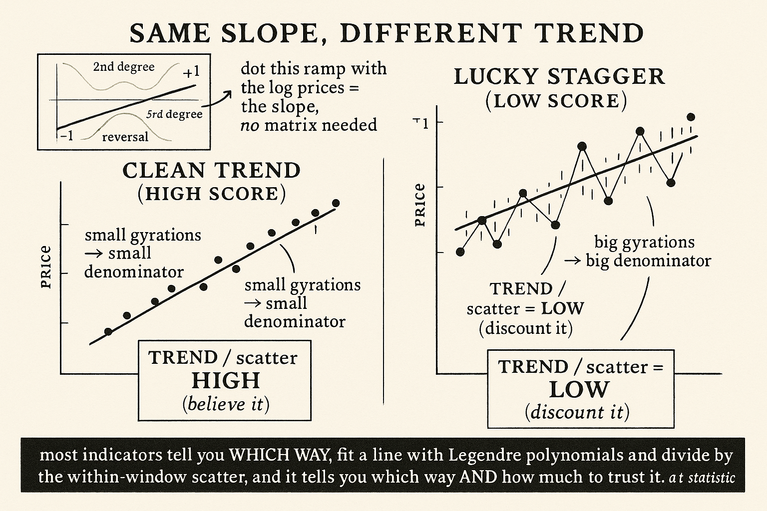
Most indicators tell you which way price went. Fit a line to the window with Legendre polynomials and divide the slope by the within-window scatter, and you get a t-statistic for trend: direction plus how much to trust it.
Ask most indicators whether the market is trending and they answer with direction: price is above its average, so up. The old article "CMMA: A Better Momentum Primitive Than Price-minus-MA Alone" already sharpened that into a volatility-scaled distance, and the old article "Decyclers: Extracting Trend by Removing Cycle Energy" pulled trend out by deleting the cyclic part of the signal. Both still describe where price sits. Neither tells you whether the move was a clean, straight climb or a drunk stagger that happened to end higher. A grinding, low-noise advance and a violent chop with the same net displacement are different trades, and you want an indicator that scores them differently. Fitting a line with Legendre polynomials, then dividing by the local scatter, does exactly that.
Trend as a least-squares slope, not a difference
Price-minus-average compares two points and calls the gap a trend. A regression uses every bar in the window. Fit a straight line to the recent log prices by least squares and its slope is a far more stable measure of direction than any single difference, because it pools all the bars instead of leaning on the endpoints. The trick is how you fit it cheaply and cleanly, and that is what Legendre polynomials buy you.
The first-degree Legendre polynomial over a lookback window is a straight ramp that runs symmetrically from negative to positive, sums to zero across the window, and is scaled to unit length. Call it the linear basis vector. Because it is centered and normalized, projecting the window of log prices onto it (the dot product) returns the slope of the best-fit line directly, with no matrix inversion and no intercept to estimate.
$$ c_1(i) = \frac{i - \bar{\imath}}{\sqrt{\sum_{j}\left(j - \bar{\imath}\right)^2}}, \qquad \text{Trend} = \sum_{i=1}^{L} c_1(i)\, \ln P_i $$
The term c-one is the normalized linear basis: i indexes the bars in the window, i-bar is the middle bar, so the numerator is just each bar's distance from center, and the denominator rescales the whole ramp to unit length. The trend is the dot product of that ramp with the log prices in the window. A steadily rising series lines up with the ramp and produces a large positive number; a falling series produces a large negative one; a flat or symmetric series cancels against the centered ramp and produces near zero. Use log prices so the slope reads as a compounding rate rather than a dollar amount, the same reason the old CMMA primitive worked in returns rather than levels.
The basis does not stop at a line. The second-degree Legendre polynomial is a centered parabola, and projecting onto it measures curvature, whether the trend is accelerating or rolling over. The third-degree one is a cubic that captures an S-shape. Each higher polynomial is orthogonal to the ones below it, so the linear, quadratic, and cubic coefficients carry independent pieces of the move and you can read slope, acceleration, and reversal as separate signals from the same fit.
Dividing by the gyrations
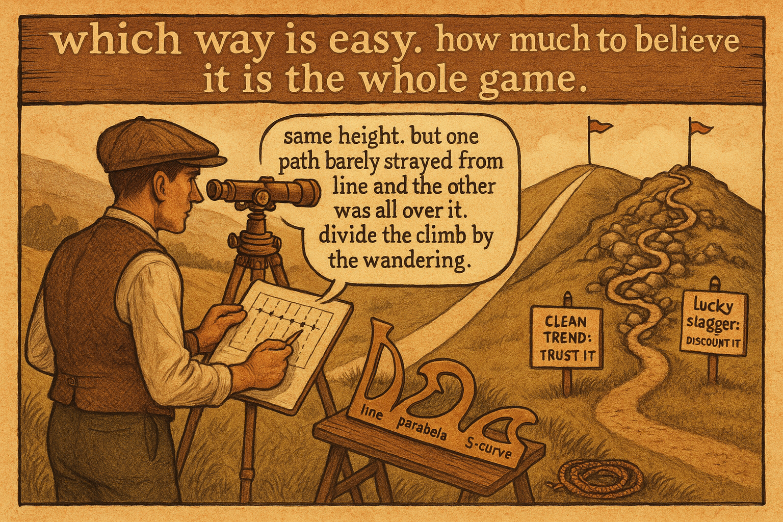
The slope alone still cannot tell the clean climb from the lucky stagger, because both can share the same slope. The information you are missing is how far the prices strayed from the fitted line along the way. A tight fit means the move tracked the line bar by bar, a real trend. A loose fit means the prices wandered all over and the line is a polite fiction. Measure that scatter as the root-mean-square of the residuals around the fit, the within-window gyrations, and divide the trend by it.
$$ \text{TrendRel} = \frac{\text{Trend}}{\sqrt{\dfrac{1}{L}\sum_{i=1}^{L}\left(\ln P_i - \widehat{\ln P_i}\right)^2}} $$
The numerator is the slope from before. The denominator is the typical distance between the actual log price and the line you fitted to it, averaged over the window. Their ratio is a signal-to-noise reading of the trend: the move scaled by how much of the window was gyration rather than progress. A clean, low-residual advance produces a large ratio even at a modest slope, while a steep but jagged move with the same displacement gets discounted by its own noise. This is the same shape as a regression t-statistic, slope over the spread of the residuals, and it answers a sharper question than "which way" — it answers "how much of this move should I believe."
Two practical notes. Raw ratios like this grow heavy tails when a near-flat window drives the denominator toward zero, so pass the result through a normal cumulative distribution function to compress the extremes into a bounded, well-behaved range, the same taming step the CMMA and moving-average-difference indicators use. And the window length is the one real choice: a short window reacts fast and reports local trend with lots of variance, a long window is stable but laggy, and the right length is the horizon you actually trade rather than a number an optimizer liked in-sample.
Where it fits against what you already have
The decyclers article got trend by subtracting the cyclic energy, a filter-side answer. This is the regression-side answer to the same question, and the two are complementary: the decycler cleans the series, the Legendre fit measures the slope and, more usefully, the conviction behind it. Against CMMA, the Legendre trend is the multi-bar generalization. CMMA scales a single displacement by volatility; the Legendre-relative trend scales a whole-window slope by the window's own scatter, so it rewards persistence and punishes chop in a way a two-point distance cannot. Use it as a regime gauge, gate other signals on it, or feed the linear, quadratic, and relative-trend values straight into a model as a compact description of the recent move that says direction, acceleration, and trustworthiness in three numbers.
Visualizing trend relative to variation
KEY POINTS
- Direction indicators say where price sits; they cannot tell a clean straight climb from a jagged stagger with the same net displacement. Those are different trades.
- Fit a line to the window of log prices by least squares: the slope pools every bar and is far more stable than any single price-minus-average difference.
- The first-degree Legendre polynomial is a centered, unit-length linear ramp. Its dot product with the log prices returns the best-fit slope directly, with no matrix inversion and no intercept to estimate.
- Higher Legendre polynomials are orthogonal: the second-degree parabola measures curvature (acceleration or roll-over) and the third-degree cubic captures an S-shaped reversal, three independent signals from one fit.
- Divide the slope by the root-mean-square of the residuals around the fit, the within-window gyrations. The ratio is a signal-to-noise reading: a clean low-residual move scores high even at a modest slope; a steep jagged move with the same displacement gets discounted by its own noise.
- The construction is the shape of a regression t-statistic, slope over residual spread, and it answers "how much of this move should I believe," not just "which way."
- Compress the ratio through a normal CDF to bound heavy tails when a flat window drives the denominator toward zero, and pick the window length as the horizon you trade.
- It is the regression-side complement to the filter-side trend of the old article "Decyclers: Extracting Trend by Removing Cycle Energy," and the multi-bar generalization of the old article "CMMA: A Better Momentum Primitive Than Price-minus-MA Alone."