4. Market Structure Notes June 27, 2026 5 min

4.49 The Hurst Exponent from Fractal Dimension

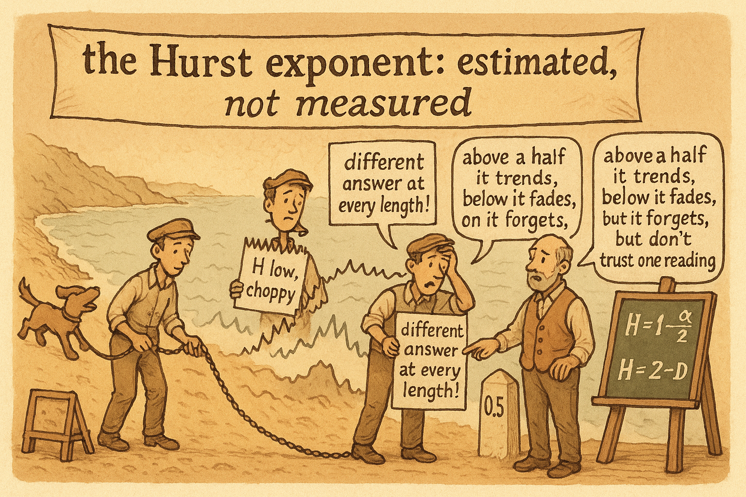
The Hurst exponent reads the same persistence axis as the efficiency ratio, linked by H = 1 - alpha/2 and H = 2 - D. But it's estimated, not computed, and drifts with data length, so read it as a profile.

The old article "Efficiency Ratio Explained for Traders" gave you one number on a zero-to-one scale that says how much of a market's motion became net direction. The old article "Variance Ratio Tests for Traders" gave you another, built from how variance grows with horizon, that says whether moves reinforce or reverse. The Hurst exponent is a third member of the same family, and the three agree more often than not because they all measure persistence. What makes Hurst worth knowing is its plumbing: it connects the spectral slope from the noise-color view to the fractal dimension of the price curve, three different measurements of one property tied together by two short equations.

Hurst lives on the same scale as the efficiency ratio

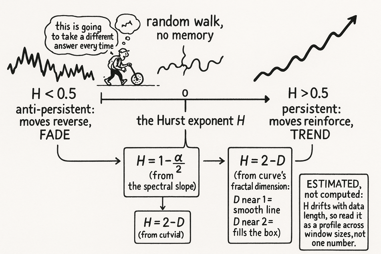
The Hurst exponent, written H, runs between zero and one, and the reading splits at one half.

$$ H < 0.5 \;\;\text{anti-persistent (mean-reverting)} \qquad H = 0.5 \;\;\text{random walk} \qquad H > 0.5 \;\;\text{persistent (trending)} $$

A market with H below one half is anti-persistent: an up move is more likely to be followed by a down move, motion cancels, and this is the fade environment the old efficiency-ratio article flagged with a low reading. A market with H above one half is persistent: moves reinforce, the trend environment. H at exactly one half is the random walk, no memory either way. This is the variance-ratio result wearing a different number; a variance ratio above one (moves reinforcing) corresponds to H above one half, and a ratio below one to H below one half. Same axis, three instruments.

Two equations connect Hurst to slope and to shape

The reason Hurst is more than a fourth redundant indicator is that it bridges the two views from the noise-color article: the spectral slope and the geometric roughness of the curve. The first bridge ties H to the spectral exponent alpha.

$$ H \;=\; 1 - \frac{\alpha}{2} $$

Recall from the old article on noise colors that alpha is the slope of the log power spectrum. White noise (alpha = 0) gives H = 1, brownian noise (alpha = 2) gives H = 0; the often-quoted "H = 0.5 is a random walk" applies to the price increments, where the bookkeeping lands at one half. The point is that you do not need a separate machine for Hurst, you can read it off the spectral slope you already estimated. The second bridge is more practical, because it ties H to the fractal dimension D of the price curve, a quantity you can measure directly off the chart without any spectrum at all.

$$ H \;=\; 2 - D $$

The fractal dimension D measures how thoroughly the wiggly price line fills the plane: a clean directional line has D near 1, a series so choppy it nearly fills its box has D near 2. So a smooth trending curve (low D, near 1) gives high H (near 1, persistent), and a jagged choppy curve (high D, near 2) gives low H (near 0, anti-persistent). The geometry of the line and its memory are the same fact. The old article on noise colors gave you the spectral route, H equals one minus alpha over two; this gives you the geometric route, H equals two minus D, and the next article shows how to get D straight off the bars.

The catch: it is estimated, not computed

Here is where most write-ups stop and most traders get burned. The efficiency ratio is computed: feed it a window and it returns an exact number. The Hurst exponent is estimated: there is no closed-form value, only a number you fit, and the fit depends on choices that move it around. Worst of all, H changes dramatically with the length of the data used. Run the estimate over 200 bars and over 2000 bars of the same instrument and you can get materially different exponents, not because the market changed but because the estimator is sensitive to scale and to the range of horizons you let it see. This is the same warning the old variance-ratio article gave from its own angle: the persistence reading is a property of the sample and the window, noisy on short samples, distorted by fat tails, and capable of vanishing out of sample.

So treat H as a regime label with error bars, never a precise constant. Report it as a profile across data lengths rather than a single figure, the way the old efficiency-ratio article insisted on a short/horizon/long reading instead of one number. If H is comfortably above one half across several window lengths, the persistence is probably real and a trend approach has structural support; if it hovers near one half or flips with window length, you are looking at a random walk dressed up by estimation noise, and any strategy keyed to it is fitting the estimator, not the market.

KEY POINTS

The Hurst exponent H runs 0 to 1: below 0.5 is anti-persistent (mean-reverting, the fade environment), 0.5 is a random walk, above 0.5 is persistent (trending). It sits on the same persistence axis as the efficiency ratio and the variance ratio.
Two equations connect it to the noise-color view: H = 1 - alpha/2 ties it to the spectral slope alpha, and H = 2 - D ties it to the fractal dimension D of the price curve.
A smooth directional curve has low fractal dimension (D near 1) and high H (persistent); a jagged box-filling curve has high D (near 2) and low H (anti-persistent). Geometry and memory are the same fact.
H is estimated, not computed: there is no exact value, only a fit, and it changes dramatically with the length of data used, echoing the variance-ratio warning that persistence readings are sample properties.
Use it as a regime label with error bars: report a profile across window lengths, trust a trend read only when H stays above 0.5 across several lengths, and distrust any reading that flips with window size as estimation noise.

Hurst lives on the same scale as the efficiency ratio

Two equations connect Hurst to slope and to shape

Subscribe to Aligrithm

The catch: it is estimated, not computed

KEY POINTS

References