4.50 Measuring Fractal Dimension Directly from Price
Fractal dimension measures choppiness as a number: count price range over interval at two scales. D near 1 is a clean trend, D near 2 is chop, and H = 2 - D hands you the Hurst reading.
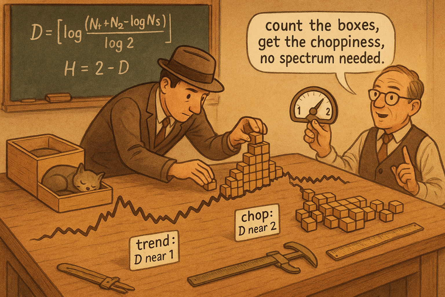
The old article "The Hurst Exponent from Fractal Dimension" left you with a promise: H equals two minus D, so if you can measure the fractal dimension D of the price curve you get the persistence reading for free, no spectrum required. This article cashes that promise. The old article "Price Density: A Visual Way to Measure Market Choppiness" already gave you the intuition, counting how many times price covers its own box, and fractal dimension is that same intuition made into a number you can compute in three lines on any bar series.
Fractal dimension by covering a shape with boxes
The textbook way to find a fractal dimension is box-counting. Cover a shape with boxes of size S, count how many boxes N it takes, then shrink the boxes and count again. The dimension is how fast the count grows as the boxes shrink.
$$ \frac{N_2}{N_1} = \left(\frac{S_1}{S_2}\right)^{D} \qquad\Longrightarrow\qquad D = \frac{\log(N_2/N_1)}{\log(S_1/S_2)} $$
Check it on shapes you know. A straight line one meter long: with one-meter boxes you need 10 to cover a ten-meter span, with tenth-of-a-meter boxes you need 100, so D equals log(100/10) over log(1/0.1), which is one. A line is one-dimensional. Do the same on a filled square and you need 10,000 of the small boxes against 100 of the large, giving D equal to two. A square is two-dimensional. A price curve is neither: it is a wiggly line stuck somewhere between dimension one and dimension two, and where it sits between them is exactly its choppiness.
The shortcut that works because bars are evenly spaced
Covering a real price curve with literal boxes is fiddly, but price has a feature that hands you a shortcut: the bars are uniformly spaced in time. With even spacing, the box count over any interval is approximately the curve's average slope over that interval, which is just the price range divided by the length of the interval.
$$ N_i = \frac{\text{Highest} - \text{Lowest}}{\text{Interval}} $$
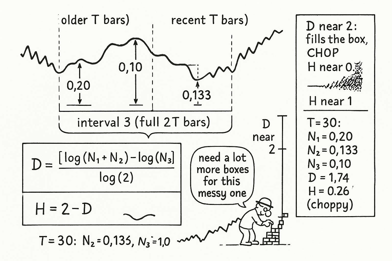
Now build the estimate from two equal windows so you have a small box and a large box to compare, the two scales box-counting needs. Take a lookback of 2T bars and split it. Interval 1 covers the most recent T bars (now back to T bars ago), interval 2 covers the older T bars (T back to 2T bars ago), and interval 3 covers the whole 2T span at once. Compute a range-over-length count for each, then combine them.
$$ N_1 = \frac{H_1 - L_1}{T}, \quad N_2 = \frac{H_2 - L_2}{T}, \quad N_3 = \frac{H_3 - L_3}{2T} \qquad\Longrightarrow\qquad D = \frac{\log(N_1 + N_2) - \log(N_3)}{\log 2} $$
The numerator compares the fine-scale count (the two short windows added) against the coarse-scale count (the one long window), and the log-base-two is there because the long window is twice the length of each short one, so S1 over S2 is two. This is Ehlers' practical fractal dimension index, and it is cheap enough to run on every bar.
A worked reading and how to interpret it
Put numbers on it. Take T equal to 30, so a 60-bar lookback. Suppose the recent 30 bars ran from a low of 100 to a high of 106, the prior 30 bars from 101 to 105, and the full 60 bars from 100 to 106. Then N1 is 6 over 30, which is 0.20, N2 is 4 over 30, which is about 0.133, and N3 is 6 over 60, which is 0.10. The sum N1 plus N2 is 0.333. D is log(0.333) minus log(0.10), all over log(2): that is log(3.33) over log(2), roughly 1.20 over 0.693, about 1.74. A dimension near 1.74 is high, close to the box-filling limit of two, so this market is choppy, and through H equals two minus D it implies a Hurst near 0.26, deep in anti-persistent territory. The reading and the geometry agree: a market whose price retraces enough to nearly fill its box is mean-reverting.
Flip the picture. If both short windows trend cleanly in the same direction, their combined range barely exceeds the full window's range, so N1 plus N2 sits close to N3, the log difference shrinks toward zero, and D drops toward one. A dimension near one is a clean directional line, H near one, the trend environment. This is the price-density measure from the old article turned into a single bounded number: high D is the wall-to-wall box of chop, low D is the white box with a diagonal smear of a trend, and you no longer have to read it by eye.
Two failure modes carry over from the old price-density and Hurst articles and deserve a flag. The estimate is jumpy on short windows, so smooth it before you act on it, and a single wide bar or a gap inflates a range and can spike D for one reading, so prefer true range and treat sudden jumps as suspect rather than as a regime change. As always, this is a measurement of the recent sample, not a forecast: it tells you what the last 2T bars looked like, and it carries the same length-dependence warning the Hurst article hammered.
KEY POINTS
- Box-counting defines fractal dimension by how fast the box count grows as boxes shrink, D = log(N2/N1) / log(S1/S2); a line gives D = 1, a filled square gives D = 2, and a price curve sits between.
- Because bars are evenly spaced, the box count over an interval is approximately range over length, N_i = (Highest - Lowest) / Interval, which turns the abstract method into a cheap per-bar computation.
- Split a 2T lookback into two T-bar halves plus the full span and combine: D = [log(N1 + N2) - log(N3)] / log(2). This is Ehlers' practical fractal dimension index.
- High D (near 2) means the curve nearly fills its box: choppy, mean-reverting, and via H = 2 - D it maps to low Hurst. Low D (near 1) is a clean trend, high Hurst. This is the old price-density measure turned into one bounded number.
- A worked T=30 example with N1=0.20, N2=0.133, N3=0.10 gives D = 1.74 and H = 0.26, deep anti-persistent territory, matching the choppy geometry.
- It is jumpy on short windows (smooth it), distorted by single wide bars and gaps (use true range, distrust spikes), and a measurement of the recent sample rather than a forecast, carrying the same length-dependence as the Hurst estimate.
References
- Cycle Analytics for Traders - John Ehlers (Amazon)
- Box-counting dimension (overview, Wikipedia)
- How Long Is the Coast of Britain? (Mandelbrot, 1967)
- The Fractal Geometry of Nature (Mandelbrot, overview)
- Fractal Dimension Index and trend-vs-range detection (practitioner note)
- Trading Systems and Methods - Perry Kaufman (Amazon)
- Cybernetic Trading Strategies - Murray Ruggiero (Amazon)
- The Art of Currency Trading - Brent Donnelly (Amazon)
- Fractal Market Hypothesis: An In-Depth Review
- Analysis on historical data of stock indices using Fractal dimension
- Hurst exponent dynamics of S&P 500 returns: Implications for market efficiency, long memory, multifractality and financial crises predictability
- Fractal properties, information theory, and market efficiency
- Applying Hurst Exponent in pair trading strategies on Nasdaq 100 stocks
- Closed Contour Fractal Dimension Estimation by the Fourier ... - arXiv
- The Omniscient yet Lazy InvestorSubmitted to the editors DATE
- The Unpredictability of Complex Systems - jstor