1.28 Model-Based or Data-Mined: Lotter's Framing of the Whole Problem

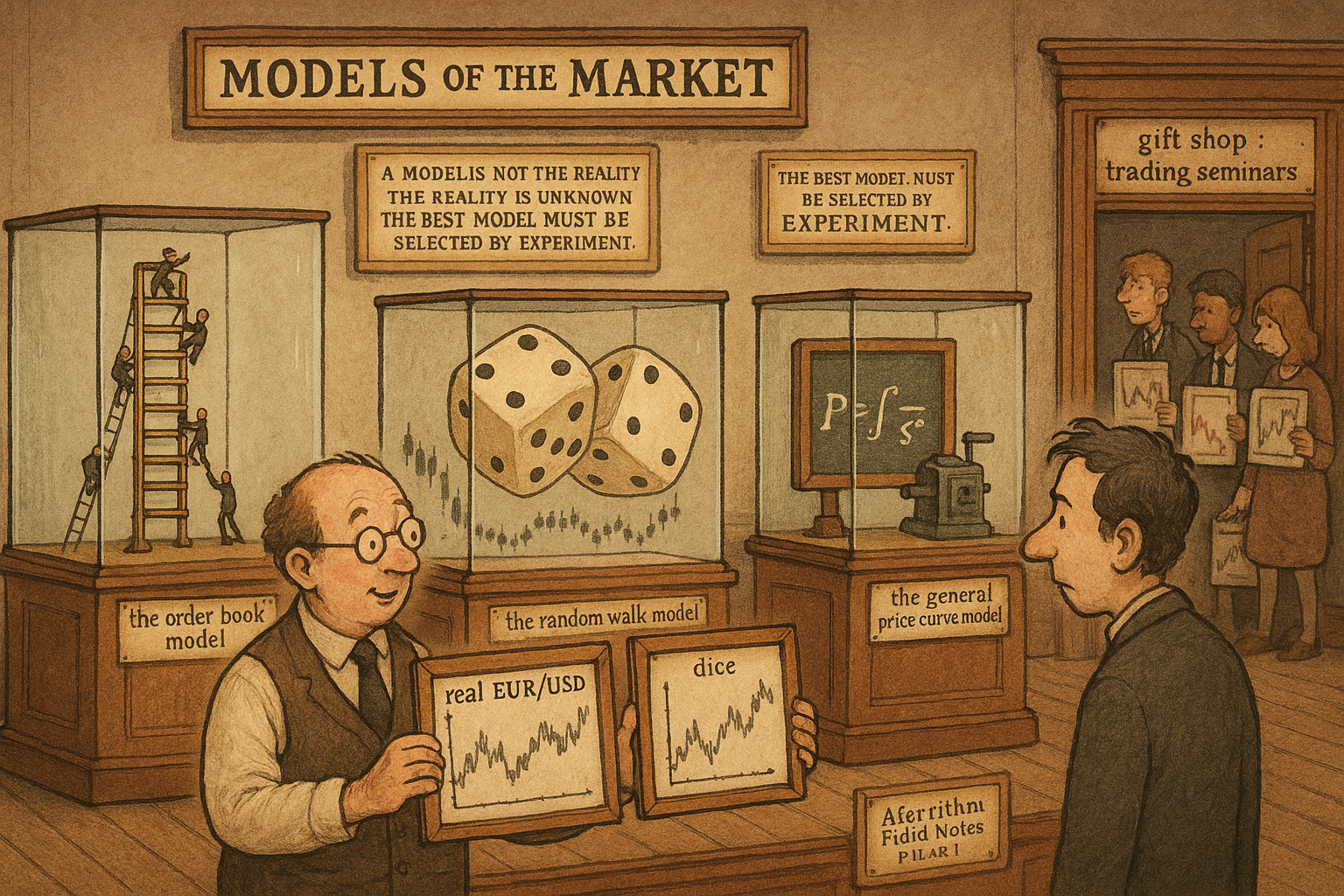
Johann Christian Lotter opens his workshop deck with four lines that do more work than most methodology chapters. A model is not the reality. The reality is unknown. The same reality can be described with many different models. The best model must be selected by experiment. Every argument in Pillar 1 reduces to those four lines, and the deck states them in under thirty words before showing a single chart.

The split he builds on top of them is the useful part. Model-based development starts with a market theory and looks for it in the data. Data mining starts with the price data and hunts for patterns that predict. Both end with a rule you can code, and the deck is honest that neither is safe. What follows takes the framing seriously, checks the arithmetic on the deck's own slides, and finds two places where the illustrations do not support the claim printed above them.

The order book model, and where its arithmetic slips

The first model is mechanical rather than statistical. Lotter puts up a book with asks of 10k at 1.03, 20k at 1.02 and 10k at 1.01, and bids of 20k at 0.99, 10k at 0.98 and 10k at 0.97. The broker quotes price 1.01 and spread 0.02, which is the best ask and the distance to the best bid. Buy 10k at market and the 1.01 level disappears. The new best ask is 1.02, the best bid is still 0.99, and the quoted price and spread become 1.02 and 0.03. A buy order pushes the price up. This is not a theory about trader psychology, it is bookkeeping.

The next slide is where the arithmetic slips. You buy 10k at market and someone else sells 10k at market. Lotter marks both the 1.01 ask and the 0.99 bid as filled, then reports the new price as 1.01 and the spread as 0.02, unchanged, with the conclusion that buy and sell orders cancel each other. Against the static book he drew, they do not. Consuming the 1.01 ask leaves 1.02 as the best offer and consuming part of the 20k at 0.99 leaves 10k there, so the quote moves to 1.02 by 0.99 and the spread widens to 0.03. His arithmetic holds only if the two market orders cross against each other rather than against the resting book, or if a dealer reposts the consumed levels straightaway. Both are reasonable assumptions about a retail forex broker, and neither appears on the slide. Keep the conclusion, which is that balanced two-way flow leaves the mid unmoved, and treat the ladder as a sketch rather than a matching engine.

The random walk is the null, and it looks exactly like a price chart

The second model is two dice. Roll one for buyers, roll one for sellers, and set the next price to the previous price plus buyers minus sellers. Lotter then plots a real EUR/USD curve against a synthetic random one and asks which is which.

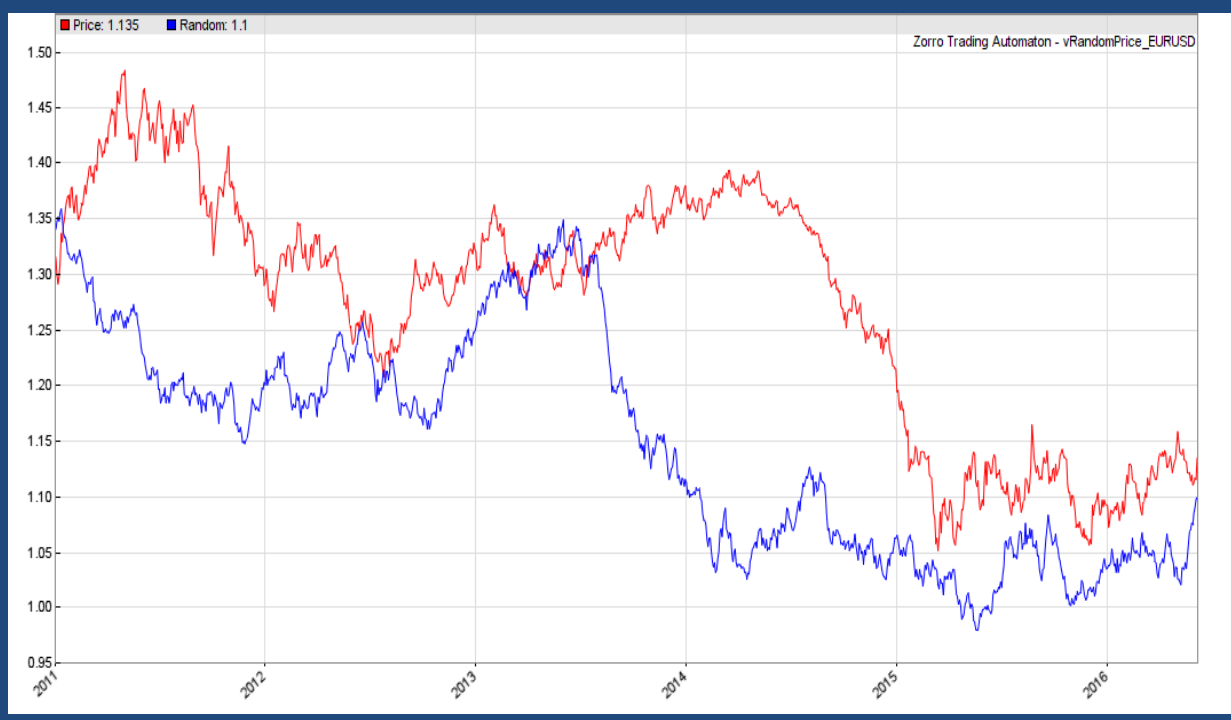
The red line is the real EUR/USD. The blue line is dice. Both trend, both consolidate, both put in what a chartist would call double tops and channel breakouts. If your rule discovery process cannot tell these two curves apart, it is not discovering anything, which is the argument the old article "The Null Hypothesis for Trading Systems" makes from the statistical side and this chart makes from the visual side.

Two rules fall out of the dice model. The first is that a pure random walk curve cannot be traded, which Lotter calls the rule of no roulette system. The second is the one people ignore.

$$ \sigma(T) \;=\; \sigma_1 \sqrt{T} $$

Volatility over T bars equals the one-bar volatility times the square root of T. This comes from adding independent increments: variances add, standard deviations add in quadrature, so the standard deviation grows as the square root of the number of steps rather than in proportion to it. Work the dice case. One fair die has variance (36 minus 1) over 12, which is 2.9167. The difference of two independent dice has variance 5.8333 and standard deviation 2.4152. After 100 rolls the spread of outcomes has standard deviation 2.4152 times 10, which is 24.15. After 400 rolls it is 2.4152 times 20, which is 48.30. Four times the duration, twice the dispersion.

The same rule on EUR/USD with a 0.6% daily standard deviation gives 0.6 times the square root of 20, which is 2.68% over a trading month, and 0.6 times the square root of 250, which is 9.49% over a year. The consequence Lotter draws is the one worth stealing. Maximum drawdown scales the same way, so a drawdown measured on a short backtest is not comparable to one measured on a long backtest. A system that showed a 12% drawdown over three years should be expected to show 12 times the square root of 2, which is 17%, over six years. Compute a Calmar ratio from a 10% annual return and the three-year drawdown and you get 0.83. Use the six-year-equivalent drawdown and you get 0.59. Skipping the normalization inflated the ratio by 41%.

Every strategy in the deck is one equation

The third model is the general one, and it is the reason the deck is worth reading twice.

$$ y_t \;=\; y_{t-1} \;+\; f\!\left(y_{t-1}, \ldots, y_{t-n}\right) \;+\; \varepsilon_f \;+\; \varepsilon_r $$

Today's price equals yesterday's price, plus a deterministic function f of the recent price history, plus a fundamental shock epsilon-f, plus a random shock epsilon-r. Set f to zero and you have the random walk. Everything a trader calls an edge lives inside f, and Lotter defines inefficiency as a systematic deviation from the random walk, which is the same thing as saying f is not zero. Roughly 99% of tomorrow's price is yesterday's price; the fight is over the remainder.

Momentum and mean reversion are two choices of f.

$$ \begin{aligned} \text{Momentum:}\quad y_t &= y_{t-1} + a_1\,(y_{t-1}-y_{t-2}) + a_2\,(y_{t-2}-y_{t-3}) + \ldots + \varepsilon_f + \varepsilon_r \\[6pt] \text{Mean reversion:}\quad y_t &= y_{t-1} - \frac{1}{\lambda}\,\bigl(y_{t-1}-\hat{y}\bigr) + \varepsilon_f + \varepsilon_r \end{aligned} $$

The momentum form says a fraction a-one of the last bar's move carries into the next bar, plus smaller contributions from older bars. The mean reversion form says the price gets pulled back toward a reference level y-hat by one over lambda of its current distance from it, so lambda sets the speed. Work the reversion case with lambda equal to 20, a reference of 1.1000 and a current price of 1.1200. The pull is one twentieth of 0.0200, which is 0.0010 against you per bar. The gap decays by a factor of 0.95 each bar, so the half-life is the log of 0.5 divided by the log of 0.95, which is 13.5 bars. The continuous approximation, lambda times the log of 2, gives 13.9. Use the discrete number when your bars are the unit you trade.

Now the momentum case, because the arithmetic there explains why so many systems die. Take a-one equal to 0.05 and hourly EUR/USD bars with a return standard deviation of 0.0010, which is 10 pips. The average absolute move is 0.8 times the standard deviation, so 8 pips, and the expected drift the momentum term buys you is 0.05 times 8 pips, which is 0.4 pips per bar. The noise on that same bar is 10 pips. Signal over noise per bar is 0.04. Because the drift accumulates in proportion to the number of bars while the noise accumulates as the square root, the ratio grows as 0.04 times the square root of N. Reaching a ratio of 2 needs the square root of N to be 50, so 2,500 bars. That is the rule of square root volatility working against you rather than for you, and it says a 5% autocorrelation is real and undetectable on a few hundred bars at the same time.

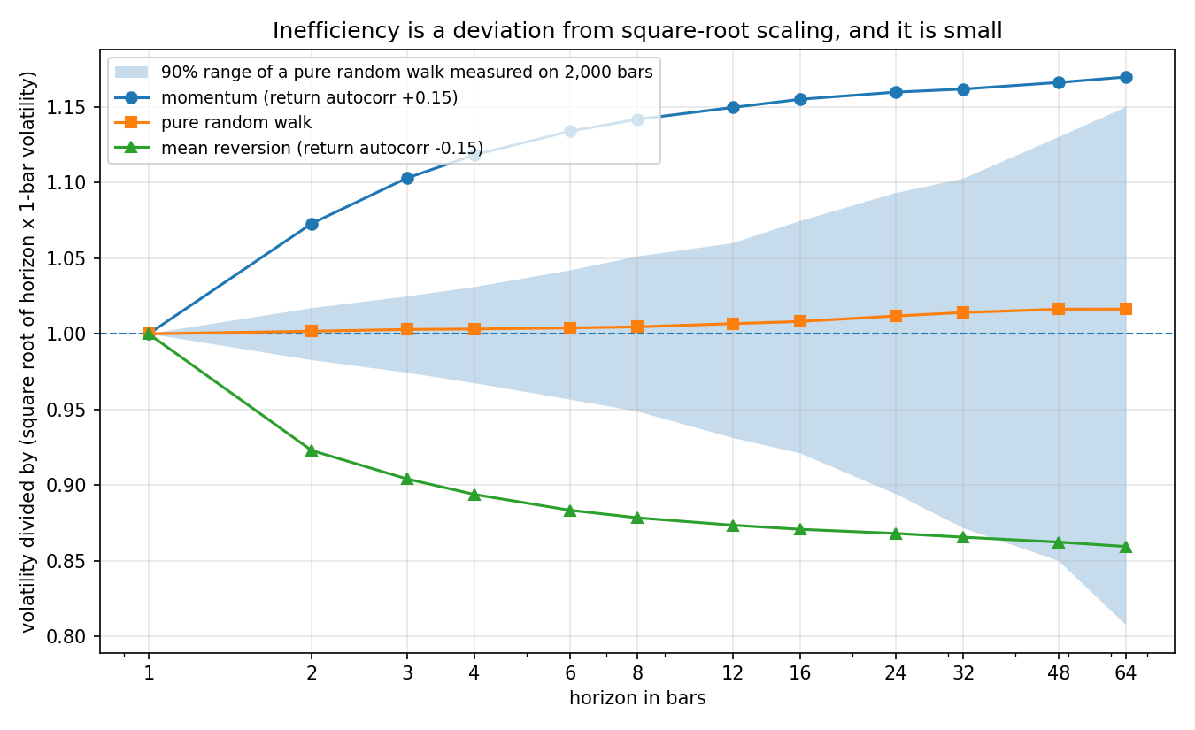
I simulated the three cases on 400,000 bars each and divided the T-bar volatility by the square root of T times the one-bar volatility, so a pure random walk sits at 1.0 by construction. The momentum series with a return autocorrelation of +0.15 climbs to 1.17 by 64 bars and the mean-reverting one falls to 0.86, while the random walk stays within 2% of the line. The shaded band is the honest part: it shows where that same statistic lands on 2,000 bars of pure dice, at the 5th and 95th percentiles across 500 draws. At a 2-bar horizon the band is narrow, roughly 0.98 to 1.02, and both inefficiencies sit far outside it. At 64 bars the band runs from 0.81 to 1.15 and swallows the mean-reverting curve whole. Two thousand bars holds only 31 non-overlapping 64-bar windows, and 31 observations cannot resolve a 14% effect. The deviation from the random walk is what you are hunting, it is small, and your ability to see it collapses as the horizon grows.

Three prerequisites, and the test the slide does not run

Lotter's bar for accepting a model has three parts. It has a rational basis in market structure or trader behavior. It can be written as a program flow or a formula. It has statistical significance in real price curves. Then the procedure: find an algorithm that detects the inefficiency, compute a statistic, plot a histogram, and compare against random walk curves or shuffled price curves. His last instruction is blunt, which is not to rely on other people's research because scam is ubiquitous. He names Elliott Waves as the example.

The illustration he chooses is a frequency spectrum of EUR/USD.

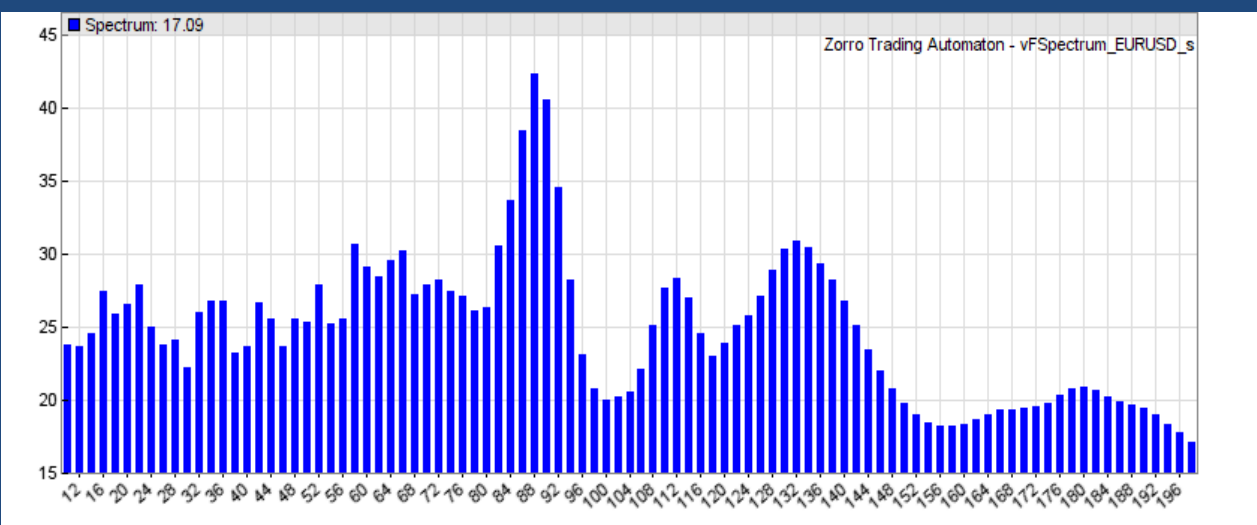
The peak sits at a period near 88 bars and reaches about 42 against a typical bar height near 25. Reading the other bars off the chart, they scatter roughly between 17 and 31, so a standard deviation near 4. That puts the peak about 4.3 standard deviations above the middle of the pack, and 11 points clear of the next tallest bar anywhere in the spectrum. With 47 bins, the largest of 47 independent draws would be expected to land about 2.2 standard deviations above the mean, so 4.3 is beyond what bin-picking alone explains, and the fact that the peak is a cluster of five adjacent tall bars rather than one spike makes it harder to dismiss.

That is my calculation, not his, and it is the calculation the slide skips. The deck tells you to compare against shuffled price curves and then shows a spectrum with no shuffled baseline on it, no confidence band, and no statement of the sample period or the number of assets scanned. A cycle detected on one currency over one window, presented without the comparison the previous slide demanded, is exactly the evidence standard the deck warns against three slides earlier.

The filter matters more than the algorithm

One line in the development process deserves more attention than the seven-step list around it. A market inefficiency does not exist all the time, so you need a filter that decides whether it is present, and in most cases the filter matters more than the algorithm.

This inverts how most people allocate their effort. The cycle strategy is four lines: detect the dominant cycle and phase, generate a forerunning sine, short at a peak, long at a valley. The filter is one line: trade only when the amplitude of the dominant cycle exceeds a threshold. The four lines are the part everyone tunes and the one line is the part that decides whether the system makes money, because a cycle system running through a trending regime bleeds on every entry. The same asymmetry shows up in the trend and reversion strategies, both of which open with the identical instruction to detect the market regime first.

His warnings on parameter fitting are the standard ones and they are correct. Do not optimize too many parameters. Do not optimize for peaks, which rules out brute force and genetic search as the final step. Find the most robust parameter range instead, the sweet spot. The old article "Why Simplicity Is a Statistical Weapon" gives the reason in statistical terms: every parameter you add hands noise another lever.

The reality check in the deck does not pass

Walk-forward analysis gets a fair treatment. Roll a window across the simulation, split it into a training and a test section, and the test is out of sample while still covering most of the data. Lotter names the cost immediately, which is that the system now depends on two more parameters, the cycle count and the split. Then he says that even after walk-forward and Monte Carlo the results still carry bias introduced by the development process itself, and he lists four ways to measure it, with White's Reality Check first.

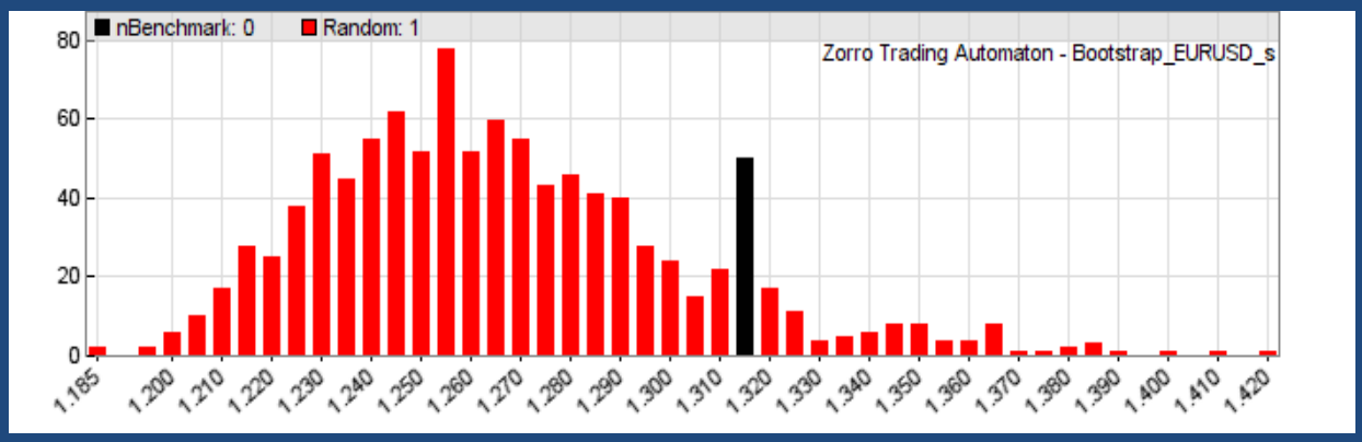
Read this chart the way the method intends. The red histogram is the strategy run on many randomized versions of the price curve, and the black bar is the real result, a profit factor near 1.32. The p-value is the fraction of red mass at or to the right of the black bar. Counting the red bars past 1.32 by eye gives roughly 85 out of about 1,000 runs, so a p-value near 0.085. That does not clear a 5% bar. The deck's own illustration of how to detect bias shows a system whose edge fails the test, and the slide does not say so.

Two more things sit in that picture. The randomized runs average a profit factor around 1.26, so the shuffled curves are profitable before any skill is involved, which is the long-bias trap in miniature. And a profit factor of 1.32 against a random mean of 1.26 is a thin margin to begin with, whatever the p-value turns out to be. I would not trade this, and I do not think the chart was chosen to be flattering. It was chosen to show the method, and the method worked.

Reinvest the square root of your profits

The money management slides carry the deck's only clean numbers, and they reward a Calmar comparison the deck itself does not run. The same EUR/USD system compounds at 15% with no reinvestment and 16% at 1% reinvestment. Push to half of OptimalF and the compound rate jumps to 48%. Reinvest only the square root of accumulated profits and it comes back to 43%.

Taken alone, half of OptimalF wins. The equity charts say otherwise. Reading the drawdown troughs off both plots, the half-OptimalF run peaks near 175,000 and takes a worst drawdown near 60,000, which is 34% of peak. The square-root run peaks near 125,000 and takes a worst drawdown near 25,000, which is 20%. Calmar for the aggressive version is 48 over 34, so 1.41. For the square-root version it is 43 over 20, so 2.15. Giving up a tenth of the compound rate bought a 52% better return-to-drawdown ratio. That is the argument for the square root rule, and it survives the arithmetic. Those trough depths are eyeballed from chart axes rather than printed in the deck, so treat the ratio as approximate and the direction as solid.

Step 1: visit trader forums

The deck closes with seven steps labelled the real development process. Find a thread about a fabulous new indicator. Code it, find the backtest disappointing, and debug. Add a trailing stop, run a day-of-week analysis, discover Tuesday is bad, add a Tuesday filter, add a midday filter, and watch the backtest profit appear. Run a walk-forward on 23 optimized parameters, and when that disappoints, try different cycle counts and bar periods until a sensational out-of-sample number arrives. Trade it live. Watch it fail. Hold seminars.

The joke has a precise structure. Every step is a legitimate technique applied in the wrong order. Walk-forward analysis is sound. Day-of-week analysis is sound. Trailing stops are sound. Running them as a search for a number that looks good converts each one into another trial in an uncounted multiple-testing experiment, which is the failure the old article "The Scientific Method for Building Trading Systems" builds its pass and fail gates to prevent.

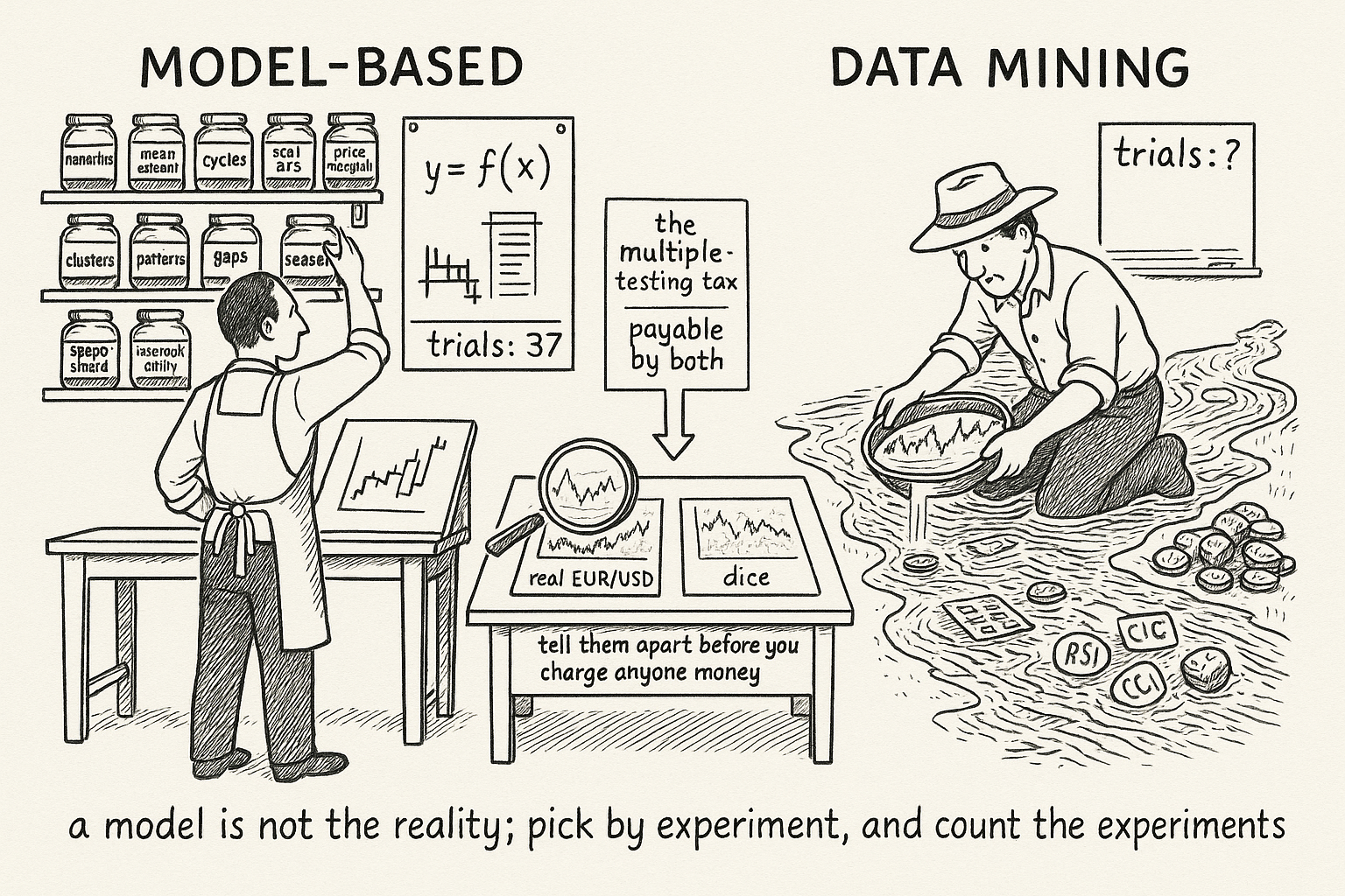
Here is where I would push back on the framing itself. Lotter presents model-based development as the disciplined alternative to data mining, and the deck's own structure undercuts that. He lists ten families of inefficiency: momentum, mean reversion, cycles, statistical arbitrage, price constraints, clusters, patterns, gaps, seasonality and heteroskedasticity. Choosing among ten models, across a handful of assets, with the best one selected by experiment, is a search over 30 or 50 specifications. The multiple-testing tax on that search is identical to the tax on mining 50 rules out of the price data. Starting from a market theory buys you a rational basis, which is worth something when you are deciding whether a survivor is plausible, and it buys you fewer free parameters inside each candidate. It does not buy you a free pass on counting your trials. The deck never counts them.

KEY POINTS

• Model-based development starts with a market theory and looks for it in the data; data mining starts with the data and hunts for patterns. Lotter's four-line epistemology sets the standard for both: a model is not reality, reality is unknown, many models fit the same reality, pick by experiment.
• The general price curve model, price equals previous price plus a function f of recent history plus a fundamental and a random shock, contains every strategy in the deck. Momentum, mean reversion, cycles and GARCH are choices of f, and inefficiency means f is not zero.
• Volatility scales as the square root of duration, so a drawdown from a three-year backtest must be multiplied by the square root of 2 before you compare it with a six-year one. Skipping that step inflated a Calmar ratio from 0.59 to 0.83 in the worked case.
• The square root rule works against detection too. A 5% momentum autocorrelation on 10-pip bars produces 0.4 pips of drift against 10 pips of noise, and needs about 2,500 bars to reach a signal-to-noise ratio of 2.
• The deck's frequency spectrum peak at 88 bars sits about 4.3 standard deviations above the other bins, which is beyond bin-picking, but it is shown with no shuffled baseline despite the previous slide demanding one.
• The White's Reality Check illustration puts roughly 85 of about 1,000 randomized runs at or above the benchmark profit factor of 1.32, so a p-value near 0.085. The deck's example of how to detect bias is a system that fails the test.
• Reinvesting the square root of profits returned 43% against 48% for half of OptimalF, with the worst drawdown falling from about 34% of peak to about 20%. Calmar goes from 1.41 to 2.15.
• Model-based development does not exempt you from the multiple-testing tax. Selecting the best of ten inefficiency families across several assets is a search with 30 or 50 trials in it, and the deck never counts them.

References

• A Reality Check for Data Snooping (White, 2000)
• Generalized Autoregressive Conditional Heteroskedasticity (Bollerslev, 1986)
• Efficient Capital Markets: A Review of Theory and Empirical Work (Fama, 1970)
• A New Interpretation of Information Rate (Kelly, 1956)
• Portfolio Selection (Markowitz, 1952)
• Model-Based Trading Strategies - Johann Christian Lotter, Financial-Hacker.com

A note on AI. The ideas, research, analysis, and conclusions in this article are my own. I use AI tools to help with editing and wordsmithing, because English is not my first language, and I am not shy about that. AI-generated ideas and AI-assisted writing are not the same thing: the first is empty slop from a generic prompt, the second is a tool for communicating years of real research more clearly. Judge the work by its substance, not by whether software helped polish the prose.