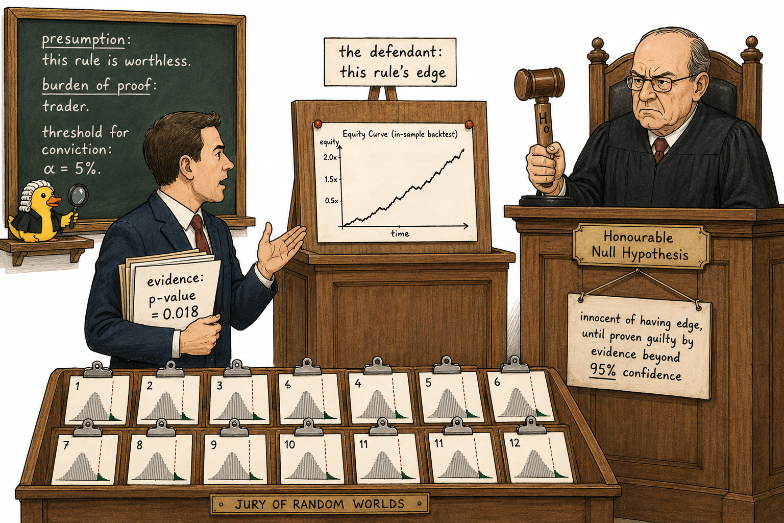
Every trading system test starts with a single sentence. The sentence is: "this rule has no predictive power." Until evidence forces a change, that sentence is the working belief. The technical name for it is the null hypothesis. Building a trading system is the process of trying to falsify the null.

The reason this matters operationally is that the null hypothesis governs every claim the trader is allowed to make. A rule that has not falsified the null is not a strategy. It is a candidate. A rule that has falsified the null is a strategy worth running. The line between the two is not the equity curve. The line is whether the backtest forced the null hypothesis into rejection.

Most retail trading research skips this step entirely. The trader runs a backtest, sees a profit, and ships. No null was stated. No falsification was attempted. The output is a hope dressed as evidence.

What the null hypothesis is

For a trading system, the null hypothesis is the formal version of "this rule is worthless." Worthless is defined precisely: the rule's expected return on detrended data is zero or negative. Detrended data removes the market's free drift, so what is left is whatever predictive content the rule actually carries.

The formal statement of the null and alternative hypotheses:

Where μ_rule^detrended is the rule's true mean return per period on detrended market data. H₀ says the rule has zero or negative edge once free drift is stripped away. H_A says the rule has positive edge. The two propositions are mutually exclusive (only one can be true) and exhaustive (one of them must be true). Falsifying H₀ logically forces H_A.

The detrending is not a cosmetic detail. A rule that holds long 90% of the time on a market that drifts up at 0.05% per day collects free return that has nothing to do with the rule. The null hypothesis applies to the part of the return the rule actually generated, which is the detrended component. Article 12 covered this decomposition.

Why H₀ is the falsification target, not H_A

This is the single most important asymmetry in hypothesis testing. The reasoning is logical, not philosophical.

H₀ is a single specific claim. It picks one value of the parameter (μ = 0) and says "the true value is this or worse." To falsify H₀, the test only has to show that the observed evidence is improbable under one specific assumption.

H_A is an infinite set of claims. The rule's true edge could be 0.001% per day, or 0.01%, or 0.1%, or anything in between or above. To falsify H_A directly, the test would have to rule out every possible positive value of the parameter. That requires an infinite number of tests. Not feasible.

So the scientific procedure is: assume H₀, see if the data forces its rejection, and accept H_A by default when H₀ falls. The asymmetry is not arbitrary. It is the only direction in which finite evidence can deliver a decision.

Why the null is assumed true at the start

Two reasons. Both are domain-independent.

The first is skepticism. The default scientific position toward any new claim is disbelief. Most claims, including most claims about trading edges, turn out to be wrong. Starting from "this rule has edge" and looking for confirming evidence is what humans do naturally and what science refuses to do. The presumption of innocence in a criminal trial works the same way. The accused is innocent until evidence proves otherwise. A trading rule has no edge until evidence proves otherwise.

The second is simplicity. Occam's razor says the simpler explanation for an observation is more likely to be correct than a more elaborate one. Two explanations exist for a profitable backtest: the rule has predictive power, or the rule got lucky in the specific sample. Luck is the simpler hypothesis. It requires no additional structure in the world. Predictive power requires an actual mechanism connecting the rule's signal to future returns. The simpler hypothesis is the default. The data has to do work to dislodge it.

Both reasons converge on the same operational rule: assume the rule is worthless until the evidence is strong enough to force a different conclusion.

The three ingredients of a hypothesis test

A complete hypothesis test for a trading rule has exactly three components. None of them are optional.

1. The null hypothesis itself. The precise statement of what the rule would do if it had no predictive power. For trading systems, the canonical form is μ_rule^detrended ≤ 0.
2. A test statistic. A single number computed on the backtest that summarizes the rule's observed performance. Mean return per signal, Sharpe ratio, hit rate, profit factor. The choice of test statistic must be made before the test runs.
3. A sampling distribution under H₀. The distribution the test statistic would take if H₀ were true. This is the hardest piece. It requires a model of what "the rule has no edge" actually looks like in terms of generated data. The model must be realistic enough to reflect the noise structure of real markets.

A test missing any of these three components is not a hypothesis test. It is a backtest with confidence theater attached.

Constructing the null model

The null hypothesis is a verbal statement. The null model is the machinery that turns it into something testable. The choice of null model is the choice that determines whether the test is rigorous or decorative.

Three levels of null model exist, in increasing order of realism.

The naive null assumes returns are independent, identically distributed normal draws with mean zero. This is what introductory textbooks teach. It is wrong for markets because real returns have fat tails, volatility clustering, and serial autocorrelation. A p-value computed against the naive null overstates the rule's significance, because the naive null underestimates how extreme outcomes can be under chance alone.

The bootstrap null resamples returns from the actual market series (after detrending) with replacement. The new series has the same marginal distribution as the real one (same mean of zero by construction, same standard deviation, same skew and kurtosis) but the time order is destroyed. Any rule that depended on the time structure of returns will produce results consistent with no edge on the bootstrap null. Any rule that produced its edge from the marginal distribution alone will look identical.

The block bootstrap null is the most realistic. It resamples blocks of consecutive returns (typically 5 to 20 days long) instead of individual days. Blocks preserve short-term autocorrelation and volatility clustering. The new series has the same marginal distribution and approximately the same dependence structure as the real one. This is the null that most trading rule tests should use.

A fourth option is the permutation null. Keep the actual market returns intact, but randomly permute the rule's signals so they fire on different days than they originally fired. This breaks the rule's specific timing claim while leaving everything else about the data unchanged. The permutation null is the cleanest test of "does this rule's signal predict anything?" because it isolates the predictive claim from everything else.

The choice of null model is not a technical detail. A bad null produces fake significance. A realistic null produces honest results, including the result "this rule has no edge that the data supports."

The decision rule

The hypothesis test rejects H₀ when the observed test statistic is improbable under H₀. The precise statement:

Where R_obs is the observed test statistic from the actual backtest, R* is the test statistic computed on a single draw from the null model, and α is the significance threshold committed to before the test ran. The standard choice is α = 0.05.

If p < α, the observed result is rare enough under H₀ that the trader rejects H₀ and accepts H_A. The rule has evidence of edge.

If p ≥ α, the observed result is consistent with what H₀ could produce by chance. The trader fails to reject H₀. The rule does not have evidence of edge. This is not the same as proving the rule has no edge. The rule might have edge that this test was not powerful enough to detect. The honest report is "we cannot reject the null at the chosen threshold," not "the rule has no edge."

Visualizing the null hypothesis test

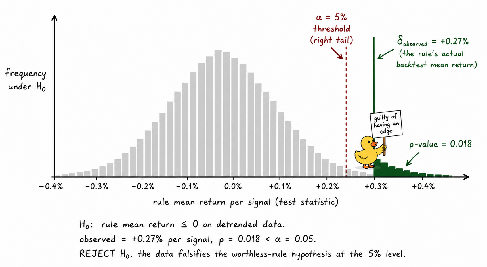
The picture is the entire null hypothesis framework in one image. The grey histogram is what the rule's performance would look like under H₀. The dashed red line is the threshold the trader committed to before running the test. The green line is what the rule produced. The shaded tail is the p-value. Crossing the dashed line is the moment of falsification.

Type I and Type II errors

Every hypothesis test can fail in two ways.

Type I error: rejecting H₀ when H₀ is actually true. The trader concludes the rule has edge when it does not. This is a false positive. The cost in trading is severe. The trader allocates capital, time, and operational complexity to a strategy that will eventually reveal it has no edge. The α threshold directly controls the Type I error rate. At α = 0.05, the trader is willing to accept a 5% probability of a false positive on any single test.

Type II error: failing to reject H₀ when H₀ is actually false. The trader concludes the rule has no edge when it does. This is a false negative. The cost is opportunity: a real edge is discarded. The Type II error rate is controlled by the test's power, which depends on the size of the true edge, the sample size, and the noise in the data.

For trading systems, Type I errors are usually more expensive than Type II errors. A worthless strategy in live trading consumes capital, attention, and confidence. A real edge that was missed costs only the opportunity. The asymmetric cost is one reason the conventional α = 0.05 threshold tends to be conservative in trading research. Some practitioners use α = 0.01 or even α = 0.005 for important live-capital decisions.

What this changes in practice

Three operational consequences follow.

Before any backtest, write down the null hypothesis, the test statistic, the null model, and the α threshold. Save the file with a timestamp. Run the backtest. Compute the p-value. Apply the decision rule. Nothing about any of these four choices can be modified after seeing the result.

Treat "fail to reject" as the default outcome. Most rules will not falsify the null. That is correct behavior, not a bug. The rules that survive a properly constructed null test are rare. Those are the rules worth trading.

Report the null test alongside the backtest performance. "Strategy returned 14% with Sharpe 1.2, p-value against block bootstrap null = 0.03" is honest. "Strategy returned 14% with Sharpe 1.2" is incomplete.

KEY POINTS

• The null hypothesis for any trading system is the formal version of "this rule has no predictive power." Operationally, μ_rule^detrended ≤ 0.
• The null and alternative hypotheses are mutually exclusive and exhaustive. Falsifying H₀ forces acceptance of H_A.
• H₀ is the falsification target because it is a single specific claim. H_A is an infinite set of claims and cannot be falsified directly.
• Two reasons justify assuming H₀ true at the start: scientific skepticism (default disbelief in new claims) and Occam's razor (luck is a simpler explanation than predictive power).
• A complete hypothesis test has three ingredients: a precise null, a defined test statistic, and a realistic sampling distribution under the null.
• The null model determines the rigor of the test. Choices, in order of realism: naive iid normal (worst), bootstrap (preserves marginal distribution), block bootstrap (preserves dependence too), permutation of signals (cleanest test of timing claim).
• Reject H₀ if p < α (typically 0.05). Otherwise fail to reject. "Fail to reject" is not the same as "accept the null." The rule might have edge the test could not detect.
• Type I errors (false positives) are usually more expensive than Type II errors (false negatives) in trading. A worthless strategy consumes capital; a missed edge only costs opportunity. Conservative α thresholds reflect this asymmetry.
• Before any backtest, commit in writing to the null, the test statistic, the null model, and the α threshold. Modifying any of them after seeing the result invalidates the test.