3. Robust Systems Lab August 21, 2026 13 min

3.41 Metaheuristics for Rule Optimization — With Diversity as the Guardrail

Four optimizers, 31 seeds, one BTC rule set. The useful output is not which one won, it is that Differential Evolution's population stayed 82% scattered after 1000 generations.

Hernández-Romo and co-authors ran four population-based optimizers 31 times each, 1000 generations per run, population of 50, tuning an eight-parameter moving-average strategy on five-minute BTC/USDC bars from January 2020 to March 2025. Differential Evolution won on average annualized return with 107.36%, against 92.05% for the Whale Optimization Algorithm, 73.47% for Particle Swarm and 61.80% for Grey Wolf. Skip that ranking. The number worth keeping sits in Section 5.4: after 1000 generations, DE's population was still 80 to 85% as spread out as the random population it started from. The search never converged onto a point, and the authors published the trace instead of hiding it.

That trace is why the paper earns a slot in a robust-systems reading list when most parameter-search papers do not. It reports how well the space got explored rather than only the best coordinate found, and that is the exact evidence a plateau argument needs. The authors then spend the conclusion ranking algorithms by peak return, which throws the evidence away. We can keep the useful half.

What they optimized, and why a grid was never an option

The strategy uses four simple moving averages, not two. SMA1 crossing above SMA2 opens a long; SMA3 crossing below SMA4 opens a short. Two independent crossover systems compete for one position slot, since the engine runs one position at a time and never holds both sides.

$$ \text{long at } t \iff SMA1_{t-2} \le SMA2_{t-2} \;\wedge\; SMA1_{t-1} > SMA2_{t-1} $$

Read it as a crossover confirmed one bar late. Two bars back the fast average sat at or below the slow one; one bar back it sat above. The signal uses bars t-2 and t-1 and fills at the close of t-1, which is how the authors keep look-ahead bias out of the fill. Worked example on a 20-period and a 90-period average: two bars back SMA1 reads 61,400 and SMA2 reads 61,550, so the first condition holds. One bar back SMA1 reads 61,620 and SMA2 reads 61,570, so the second holds. You buy at 61,620.

Exits run on multiplicative trailing levels. With the long stop factor k-sub-sll set to 0.95, that entry puts the stop at 61,620 times 0.95, or 58,539. Price runs to 68,000 and the stop ratchets to 64,600. Price falls back and the stop stays put.

Eight parameters carry the strategy: four average lengths on [5, 200] and four exit factors, the long take-profit on [1.0, 1.3], the long stop on [0.9, 0.99], the short take-profit on [0.9, 0.99] and the short stop on [1.0, 1.1]. Grid the lengths at integer resolution alone and you get 196 to the fourth power, or 1,475,789,056 combinations, before touching the four continuous factors. Each evaluation means a full backtest over five-minute bars. That arithmetic is the honest case for a population-based search, and the authors make it.

Costs are stated: 5 basis points per transaction, 1x leverage, 100% of capital per position, one order live at a time.

The objective function rewards volatility

Here is what the optimizers actually maximize.

$$ \mu(x) = \frac{1}{M}\sum_{j=1}^{M} r^{(j)}(x) \qquad f(x) = \mu(x) \;\;\text{maximised} \qquad g(x) = \max_{t} D_t - D_{\text{threshold}} \le 0 $$

The fitness of a parameter vector x is the plain average of the returns it earns across M training windows. The constraint g rejects any configuration whose longest trade exceeds D-threshold, set to five days or 432,000 seconds. Training covers January 2020 through December 2022, 36 months, with an 8-month window sliding in 4-month steps, so windows start at months 0, 4, 8 and on through 28 and M equals 8.

Worked example. Say a configuration returns 40%, 10%, -25%, 60%, 5%, -10%, 30% and 20% across those eight windows. The sum is 130, so mu equals 130 divided by 8, or 16.25%.

Now watch what that objective prefers. A configuration that gains 100% in one window and loses 50% in the next scores an average of 25%, while the account ends exactly where it started: 2.0 times 0.5 equals 1.0. A steadier configuration that gains 12% in both windows scores 12% and compounds to 1.12 squared, or 25.44%. The objective ranks the flat account above the one that made a quarter of your money. Arithmetic averaging of window returns pays for variance.

The authors open the paper by criticizing the literature for judging strategies on absolute return while ignoring volatility and drawdown. Then f(x) is absolute return. Sharpe and Sortino show up in the reporting tables and never in the objective. You get what you optimize, and they optimized the thing they said was insufficient.

The constraint has its own tell. DE's best configuration held trades for an average of 39 days in the validation period. The five-day cap binds on training trades only, so there is no formal contradiction, and the filter meant to exclude long holds still selected a configuration whose live behavior is long holds. The paper does not mention it.

Rolling windows here are an averaging device, not a walk-forward

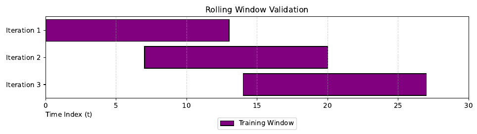
Three horizontal bars labelled Iteration 1, 2 and 3, each a fixed-length training window sliding forward in time with roughly 50 percent overlap, and a legend containing only one entry, Training Window

Look at the legend. One category: Training Window. No test block follows any of the three bars. All eight windows sit inside the 2020 to 2022 block and every one of them feeds the objective, then a single holdout runs from January 2023 to March 2025.

That design is worth something. Averaging across eight overlapping periods stops a configuration from winning on one lucky quarter, which is a robustness objective and a good one. It is not walk-forward validation, which fits on a window and then tests on the block immediately after it before rolling. The authors cite the walk-forward literature and use the term anyway. Call the scheme what it is: multi-period in-sample averaging plus one holdout. The 50% overlap also means each middle month enters the objective twice while the first and last four months enter once, so the sample's midsection carries double weight.

Diversity, the part worth stealing

The authors track a population-spread statistic every generation, following Hussain and co-authors.

$$ Div = \frac{1}{l \cdot n} \sum_{d=1}^{l} \sum_{i=1}^{n} \left| \bar{x}^{d} - x_{i}^{d} \right| $$

For each dimension d, take the population mean along that dimension, measure how far every individual sits from it, and average the whole thing over n individuals and l dimensions. Worked example on one dimension with a population of 50. If 25 individuals carry an SMA1 length of 20 and 25 carry 180, the mean is 100 and each individual sits 80 away, so that dimension contributes 80. Collapse all 50 onto a length of 45 and it contributes 0. Here n is 50 and l is 8.

They then convert the raw spread into two percentages.

$$ XPL\% = \frac{Div}{Div_{max}} \cdot 100 \qquad XPT\% = \frac{\left| Div - Div_{max} \right|}{Div_{max}} \cdot 100 \qquad XPL\% + XPT\% = 100\% $$

Div-max is the largest spread observed during the run, which lands at generation 1 when the population is still a random draw. So XPL% reads as a percentage of the initial random scatter, and XPT% is whatever remains. Worked example: a population whose spread has fallen to 12.2 from a starting 24.4 reports 50% exploration and 50% exploitation. A population at 82% exploration in generation 1000 is still 82% as scattered as the random draw it began with.

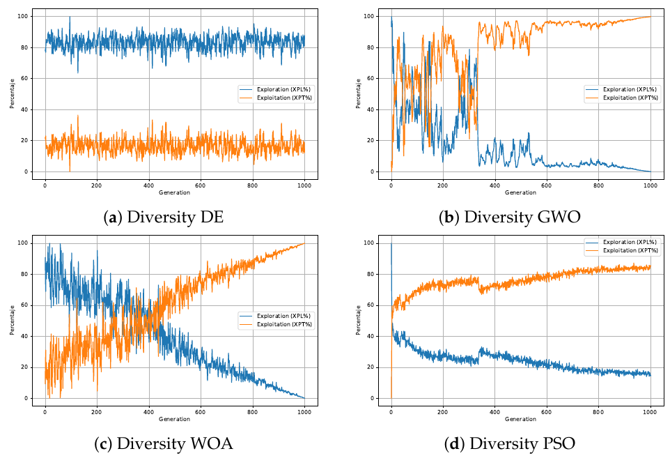
Four line charts, one per optimizer, plotting exploration and exploitation percentages across 1000 generations: DE holds exploration near 82 percent throughout, GWO and PSO see exploration collapse early, WOA hands over from exploration to exploitation in a straight line

DE runs flat at 80 to 85% for all 1000 generations. GWO thrashes for roughly 350 generations and then exploration falls to near zero, and PSO settles around 15 to 20% after an early collapse. WOA does the textbook thing, a smooth linear handover that reaches full exploitation right at the end.

A flat exploration line is a plateau statement

Fitness stopped improving in DE's runs long before generation 1000, yet the population stayed spread out. Parameter vectors sitting hundreds of bars apart in SMA length were scoring the same. That is a fitness surface with many separate basins of near-equal quality, and it is the same claim the old article "Parameter Stability Beats Best Parameter" makes from the other direction: the peak of an in-sample surface is a sampling artifact, and the thing to ship is a region.

The old article "Optimization Comes After Testing, Not Before" argues the same point procedurally, that a search which reports only its argmax has thrown away the diagnostic you needed. A diversity trace is that diagnostic, delivered for free by any population-based method, because the population is already a sample of the competitive region. Nobody has to build a separate stability map. Log the spread and read it.

One caution the authors skip. A persistently high spread has a second explanation: a flat, noisy fitness surface exerts weak selection pressure, so the population drifts rather than occupying distinct optima. The paper picks the flattering reading, "multiple distant yet competitive optima." Both readings hand a trader the same instruction. No single parameter vector is special, so do not ship one.

The metric adds bars to ratios

The equation above sums absolute deviations across dimensions with no per-dimension scaling. Four of those dimensions are moving-average lengths measured in five-minute bars with a range of 195. The other four are dimensionless exit multipliers with ranges from 0.09 to 0.30. The sum adds bars to ratios, and the units do not cancel because there are no units to cancel against.

Work out the damage. For a population spread uniformly across a range [a, b], the mean absolute deviation from the centre is (b minus a) divided by 4. Each SMA length contributes (200 minus 5) over 4, or 48.75, and four of them contribute 195.0. The long take-profit contributes 0.30 over 4, or 0.075. The long stop and the short take-profit contribute 0.09 over 4, or 0.0225 each. The short stop contributes 0.10 over 4, or 0.025. All four exit factors together contribute 0.145.

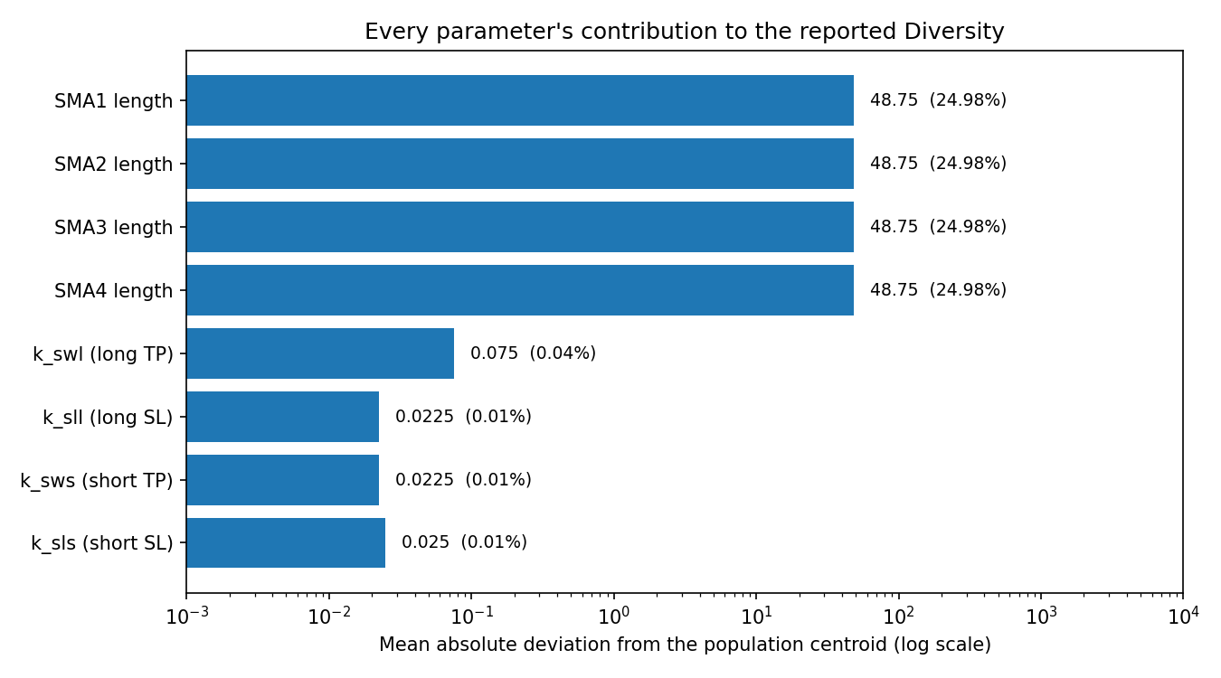
Horizontal bar chart on a log axis showing each of the eight parameters' contribution to the diversity sum: the four SMA lengths each contribute 48.75, about 25 percent apiece, while the four exit factors contribute between 0.0225 and 0.075, about 0.01 to 0.04 percent apiece

Div comes to 195.145 divided by 8, or 24.39, and the exit factors supply 0.145 of 195.145, which is 0.07% of the total. DE's 82% exploration is a statement about SMA lengths and close to nothing else. Whether the optimizer explored the stop-loss and take-profit factors, the four parameters that set the risk profile of every trade, the metric cannot say.

The fix costs one line: divide each dimension by its range before summing, so every parameter contributes on a 0 to 1 scale. Then the percentage means what the paper claims it means. Anyone borrowing this diagnostic should normalize first.

The best-of-31 column measures dispersion, not skill

Table 5 reports an average and a best across the 31 seeds. Averages run 61.80% to 107.36%, a spread of 45.56 points. The bests run 116.79% to 121.48%, a spread of 4.69 points. Four optimizers with wildly different averages produce peaks within five points of each other, and that is what the arithmetic of a maximum predicts.

$$ E\left[\max_{1 \le i \le n} X_i\right] \;\approx\; \mu + \sigma \cdot \Phi^{-1}\!\left(\frac{n - 0.375}{n + 0.25}\right) $$

For draws from a normal distribution, the expected maximum of n of them sits a fixed number of standard deviations above the mean, and that multiplier grows with n. This is Blom's approximation. With n equal to 31, the fraction is 30.625 over 31.25, or 0.98, and the inverse normal of 0.98 is 2.05. So the best of 31 seeds should land about 2.05 sigma above the average, and the gap between the two columns backs out the seed-to-seed sigma.

Run it on all four. DE's gap of 119.62 minus 107.36 is 12.26, so sigma is 12.26 over 2.05, or 6.0. WOA gives 26.10 over 2.05, or 12.7. PSO gives 48.01 over 2.05, or 23.4. GWO gives 54.99 over 2.05, or 26.8.

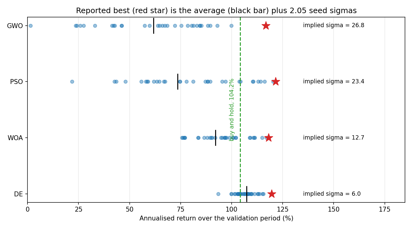
Strip plot of 31 simulated seed outcomes per optimizer using the implied sigmas, with the reported average marked by a black bar, the reported best by a red star, and a dashed green line at the 104.2 percent annualized buy-and-hold return

The back-out agrees with the paper's own claim that DE showed the lowest dispersion across runs, which is a small numerical check that passes and makes the rest of the reading safer. DE's seeds cluster inside a sigma of 6 while GWO's scatter across 27, a factor of four and a half.

That is DE's actual result. It is not that DE finds better parameters. Its peak of 119.62% is second to PSO's 121.48%. DE is the optimizer you can rerun on Tuesday and get Monday's answer from, which for anyone re-optimizing on a schedule matters more than a peak.

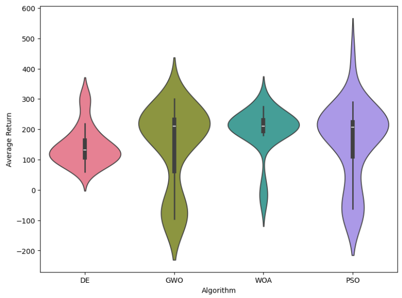
Violin plot of average return per optimizer showing DE with the narrowest distribution but the lowest median, while GWO, WOA and PSO have wider distributions with long negative tails

The violin plot confirms the dispersion story and contradicts the ranking. DE's shape is the tightest and its long tail into negative territory is missing, which is the point. Its median sits lowest of the four, around 130 on an unlabelled axis, while Table 5 hands DE the highest average. Take the picture for the widths and treat the levels as unresolved against the tables.

Two more discrepancies belong on the record. Table 5's best column and Table 7's best execution both claim to report the highest validation return per optimizer, and they agree only for GWO at 116.79%. DE reads 119.62% against 108.86%, WOA 118.15% against 120.28%, PSO 121.48% against 110.84%. Keep both as printed rather than picking one. Separately, the authors select Table 7's configurations by highest validation-period return, so the holdout did the choosing, and Table 7's Sharpe of 1.086 and its drawdown of -28.66% are in-sample with respect to that selection.

The benchmark comparison collapses under the paper's own formula

The claim: "All optimized strategies significantly outperformed a passive Buy and Hold (397.93%) benchmark." That 397.93% is cumulative over the validation window. The strategy figures, 107.36% and 120.28% and the rest, are annualized. Put them on one clock using Equation 20 from the paper itself.

$$ r_{annual} = (1 + r)^{365/d} - 1 $$

Take the total return r over d calendar days and stretch it to a year. Worked example on the benchmark. The validation period runs 1 January 2023 through 31 March 2025, which is 365 plus 366 plus 90, or 821 days. With r equal to 3.9793, the base is 4.9793 and the exponent is 365 over 821, or 0.4446. That gives 4.9793 to the power 0.4446, which is 2.042, so the annualized buy-and-hold return is 104.2%.

Against 104.2%, DE's average of 107.36% clears the benchmark by 3.2 points while carrying 108.85% annualized volatility. WOA at 92.05%, PSO at 73.47% and GWO at 61.80% all lose to holding the coin. Only the cherry-picked best runs beat it with any margin, and those are max-of-31 statistics selected on the holdout.

The paper never reports buy-and-hold's Sharpe, Sortino or maximum drawdown. For a study whose stated contribution is that prior work compares raw returns and ignores risk, omitting the benchmark's risk metrics repeats the exact failure it set out to correct. And the reproducibility section states a "356 day trading year" two lines above an equation using 365.

KEY POINTS

Log the population spread every generation and report it. Any population-based optimizer gives you a sample of the competitive region for free, so you never need a separate stability map. DE held 80 to 85% exploration for all 1000 generations, meaning parameter vectors far apart in the space scored the same.
A flat exploration line says the surface has many equal basins, which is the plateau argument from the old article "Parameter Stability Beats Best Parameter" arriving from the search side. The second explanation, a flat noisy surface with weak selection pressure, leads to the same instruction: ship a region, not a point.
Normalize each dimension by its range before summing the diversity. Unnormalized, the four SMA lengths supply 195.0 of the 195.145 total and the four exit factors supply 0.07%, so the reported percentage says nothing about whether the stop and take-profit parameters got explored.
Best-of-31 is a dispersion statistic. Blom's approximation puts the expected maximum at 2.05 sigma above the mean for 31 draws, which backs out seed sigmas of 6.0 for DE, 12.7 for WOA, 23.4 for PSO and 26.8 for GWO. Averages spread over 45.56 points collapse to peaks spread over 4.69.
DE's real advantage is reproducibility, not return. Its peak of 119.62% trails PSO's 121.48%, and its seed sigma of 6.0 beats GWO's 26.8 by a factor of four and a half. Rerun DE and you get roughly the same answer.
Optimize the metric you claim to care about. The objective is the arithmetic mean of window returns, which scores a configuration that doubles then halves at 25% while the account ends flat, and a steady 12% twice at 12% while it compounds to 25.44%. Sharpe and Sortino appear only in the reporting tables.
Annualize the benchmark before comparing. The 397.93% buy-and-hold is cumulative over 821 days, which is 104.2% annualized by the paper's own Equation 20. Three of the four optimizers lose to it on average, and the study never reports the benchmark's Sharpe, Sortino or drawdown.

References

A note on AI. The ideas, research, analysis, and conclusions in this article are my own. I use AI tools to help with editing and wordsmithing, because English is not my first language, and I am not shy about that. AI-generated ideas and AI-assisted writing are not the same thing: the first is empty slop from a generic prompt, the second is a tool for communicating years of real research more clearly. Judge the work by its substance, not by whether software helped polish the prose.

References

- Storn, R. and Price, K. (1997), Differential Evolution: A Simple and Efficient Heuristic for Global Optimization over Continuous Spaces, Journal of Global Optimization 11, 341-359
- Kennedy, J. and Eberhart, R. (1995), Particle Swarm Optimization, Proceedings of ICNN'95, 1942-1948
- Mirjalili, S. and Lewis, A. (2016), The Whale Optimization Algorithm, Advances in Engineering Software 95, 51-67
- Mirjalili, S., Mirjalili, S.M. and Lewis, A. (2014), Grey Wolf Optimizer, Advances in Engineering Software 69, 46-61
- Hussain, K., Zhu, W. and Mohd Salleh, M.N. (2019), Long-Term Memory Harris' Hawk Optimization for High Dimensional and Optimal Power Flow Problems, IEEE Access 7, 147596-147616
- Morales-Castañeda, B., Zaldívar, D., Cuevas, E., Fausto, F. and Rodríguez, A. (2020), A Better Balance in Metaheuristic Algorithms: Does It Exist?, Swarm and Evolutionary Computation 54, 100671
- Brock, W., Lakonishok, J. and LeBaron, B. (1992), Simple Technical Trading Rules and the Stochastic Properties of Stock Returns, Journal of Finance 47, 1731-1764
- Fama, E.F. and Blume, M.E. (1966), Filter Rules and Stock-Market Trading, Journal of Business 39, 226-241
- Cerqueira, V., Torgo, L. and Mozetič, I. (2020), Evaluating Time Series Forecasting Models: An Empirical Study on Performance Estimation Methods, Machine Learning 109, 1997-2028
- Suhonen, A., Lennkh, M. and Perez, F. (2017), Quantifying Backtest Overfitting in Alternative Beta Strategies, Journal of Portfolio Management 43, 90-104
- Hernández-Romo, K., Lemus-Romani, J., Vega, E., Becerra-Rozas, M. and Romo, A., Robust Metaheuristic Optimization for Algorithmic Trading: A Comparative Study of Optimization Techniques, Mathematics 2026, 14, 69