3.39 Does Complexity Actually Help? The Virtue-of-Complexity Autopsy

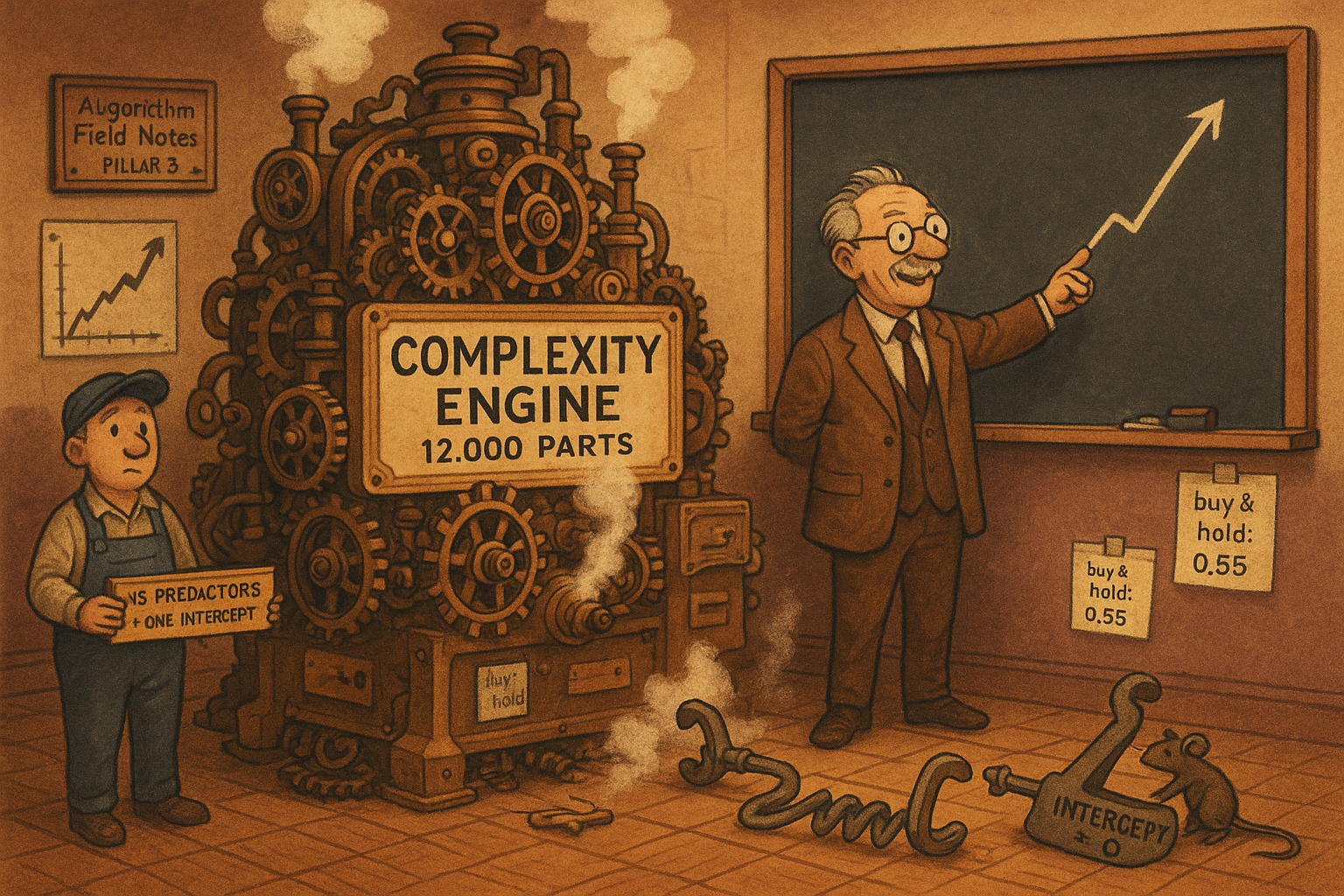
Kelly, Malamud and Zhou opened their Journal of Finance paper by reporting out-of-sample market timing Sharpe ratio improvements "relative to market buy-and-hold" of roughly 0.47 per year, earned by a model with 12,000 predictors trained on 12 monthly observations. Daniel Buncic re-ran it on the same data with the same code and found the first problem in the first sentence. Buy-and-hold on that same standardized return series earns 0.5494 over the common evaluation window. The complex model earns 0.4851. It does not improve on buy-and-hold by 0.47. It loses to buy-and-hold by 0.06, before anyone pays a spread.

That reads like a gotcha, and on its own it would be one. The substance is what Buncic does next. He shows that the headline theoretical prediction, that portfolio performance is strictly increasing in model complexity, only appears in the data because of two choices Kelly, Malamud and Zhou made in their implementation. Remove either one and the curve flattens or reverses. Neither choice has anything to do with complexity.

The machinery you need to hold in your head

The target is the excess return on the value-weighted CRSP market index, divided by a trailing 12-month volatility estimate. Call it R. The predictor set is the 15 Goyal-Welch variables, which is the standard equity premium prediction panel, plus last month's excess return. Sample runs December 1929 to December 2020 after standardization.

The random Fourier feature trick converts those 15 predictors into as many regressors as you want. Draw a random 15-by-1 weight vector omega from a standard normal, form the dot product omega-transpose G, and feed it through a sine and a cosine. Each draw manufactures a pair of new signals out of the same underlying information. Draw 6,000 times and you have P equals 12,000 regressors built from 15 variables. Nothing new enters the information set. Only the parameter count grows.

Fit by ridge regression, with shrinkage z:

$$ \hat{\beta}(z) = \left( zI + \frac{1}{T}\sum_{t=1}^{T} S_t S_t' \right)^{-1} \frac{1}{T}\sum_{t=1}^{T} S_t R_{t+1} $$

Read the middle term as the sample covariance between the regressors and next month's return, and the inverted term as the regressor covariance matrix with z added down the diagonal. Larger z pushes the coefficients toward zero. Worked scalar example, one regressor, with the regressor's mean square equal to 1 and its covariance with next month's return equal to 0.20. At z equals 0 the coefficient is 0.20 divided by 1, so 0.20. At z equals 6 it is 0.20 divided by 7, so 0.0286. At z equals 1000 it is 0.20 divided by 1001, so 0.0002. That last number matters, because Kelly, Malamud and Zhou evaluate their 15-predictor linear benchmark at only two shrinkage settings, z equals 0 and z equals 1000. On 15 predictors, z equals 1000 does not regularize the benchmark. It deletes it.

Forecasts become positions directly. The predicted return is the portfolio weight.

$$ \pi_t = \hat{R}_{t+1|t}, \qquad R^{\pi}_{t+1} = \pi_t R_{t+1} $$

You size your bet at the size of your forecast, then earn the forecast times the realization. Worked example: forecast plus 0.30 against a realized plus 1.20 pays 0.36. Forecast minus 0.30 against a realized minus 1.20 also pays 0.36, because two negatives multiply to a positive. Being confidently right in either direction pays; being confidently wrong costs the same in reverse.

Complexity is the ratio of parameters to training observations.

$$ c = \frac{P}{T} $$

With P equals 12,000 and T equals 12, c is 1000. With P equals 200 and T equals 120, c is 5/3. Hold that second identity, because it does the work later: lengthening the training window lowers complexity even when the model is unchanged. So "Sharpe ratio increases with T" and "Sharpe ratio increases as complexity falls" are the same sentence.

Choice one: a regression forced through the origin

Kelly, Malamud and Zhou fit every model without an intercept. Their footnote 35 defends it by saying that when they do add a constant, it gets shrunk so heavily that nothing changes. That defence contains the bug. Ridge penalizes the intercept along with everything else, and the intercept is the one coefficient you should never penalize, because it carries the unconditional mean of the target.

The target here has a mean of 0.1590 with a robust standard error of 0.0336, so a t-statistic of 4.47. It is not zero and the data say so loudly. None of the 15 predictors has a zero mean either. Force the fit through the origin and the model has to manufacture that non-zero mean out of slope coefficients on non-zero-mean regressors, which is a job the slopes were not hired for.

The damage shows in the bias decomposition. With the zero-intercept restriction, squared bias in the forecasts from the headline model runs between 0.0130 and 0.0267 across the three training windows. Let the intercept float and exclude it from the penalty, and squared bias drops below 0.0002 in all three. That is a reduction of at least 65-fold, and it is not the bias that ridge shrinkage is supposed to buy you in exchange for lower variance. It is bias that a modelling restriction put there.

Then the ordering flips. Estimated without an intercept, the whole Sharpe ratio surface for the random-feature models shifts down as the training window grows: 0.4888 at T equals 12, 0.4392 at T equals 60, 0.4305 at T equals 120. Shorter training window, higher complexity, better performance, exactly as advertised. Estimated with an intercept, the same surface shifts up with the training window: 0.4745, 0.5157, 0.5863. The best random-feature model in the entire exercise uses P equals 200 features on T equals 120 observations, which is a complexity of 1.67, and it is the only one that beats buy-and-hold.

Choice two: averaging Sharpe ratios instead of averaging forecasts

The random Fourier feature construction is random, so Kelly, Malamud and Zhou draw 1,000 independent sets of features and produce 1,000 forecasts for every month. Something has to collapse those into one number. They do it two different ways in the same paper.

$$ \overline{SR} = \frac{1}{N}\sum_{n=1}^{N} SR\!\left(R^{\pi,(n)}\right) \qquad\text{versus}\qquad SR^{*} = SR\!\left(\frac{1}{N}\sum_{n=1}^{N} R^{\pi,(n)}\right) $$

On the left, score each of the 1,000 draws separately and average the 1,000 scores. That is what produces the virtue-of-complexity plots in their Figures 7 through 9. On the right, average the 1,000 strategies into one portfolio and score that. That is what produces their Table I, and it is the only one of the two you could trade, since holding 1,000 separate books and averaging their Sharpe ratios is not a portfolio. Expected return and alpha are linear, so both routes give identical answers for those. Sharpe ratio, information ratio, alpha t-statistic and R-squared are nonlinear, and the two routes diverge hard at low complexity.

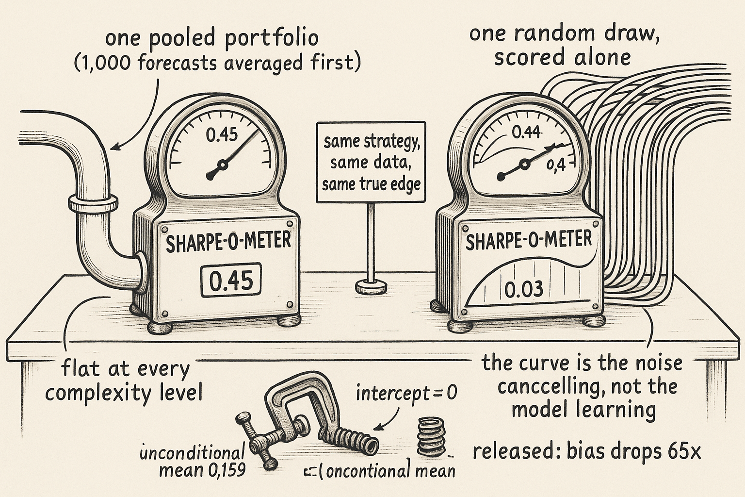
Here is why the divergence has to grow the way it does, and this mechanism is my reading rather than something the paper spells out. A single draw with P features already averages P/2 independent feature pairs inside itself. Its idiosyncratic error therefore shrinks roughly like one over the square root of P. Scoring one draw at a time means scoring a noisy strategy at small P and a self-averaged one at large P. Scoring the pooled portfolio averages across 1,000 draws no matter what P is, so it is quiet everywhere.

Put numbers on it. Let each draw's monthly timing return be a common component with mean 0.1299 and standard deviation 1, plus idiosyncratic noise of standard deviation 21.2 divided by the square root of P. The true annualized Sharpe ratio of the signal is 0.1299 divided by 1, times the square root of 12, so 0.45, and it never changes with P. At P equals 2 a single draw has standard deviation equal to the square root of 1 plus 224.7, so 15.02, and an annualized Sharpe ratio of 0.1299 divided by 15.02 times the square root of 12, so 0.030. At P equals 12,000 the same draw has standard deviation 1.019 and a Sharpe ratio of 0.44. Average those per-draw scores and you trace a curve climbing from 0.03 to 0.44, monotone and concave, on a strategy whose predictive content is constant by construction.

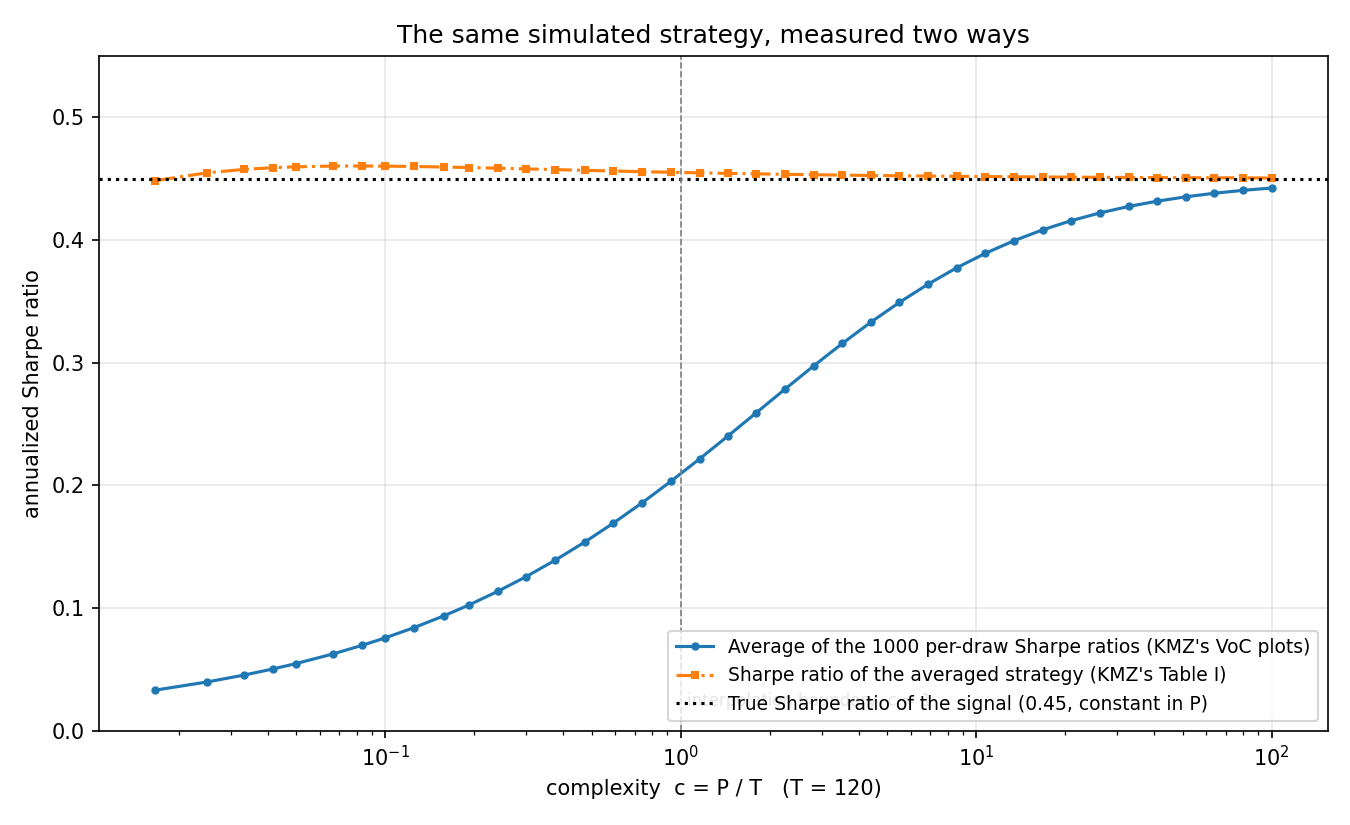
Compare the shape against the real thing. Buncic replicates both aggregations on the actual data. The solid lines are the per-draw averaging that generates the published virtue-of-complexity curves. The dash-dotted lines are the pooled portfolio.

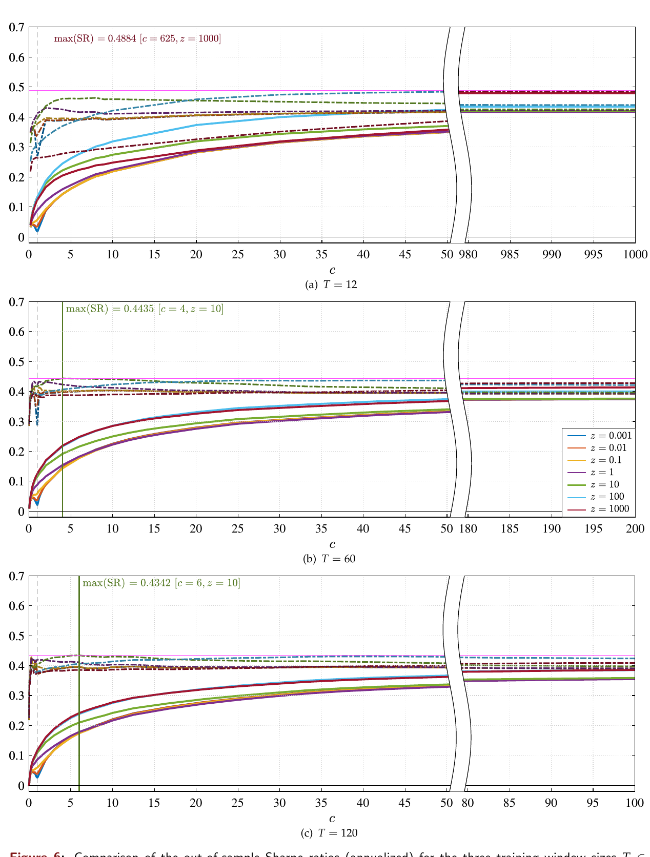
The dash-dotted lines sit above the solid lines at every level of complexity and every level of shrinkage, and they are close to flat. The rise in the solid lines is the measurement catching up, not the model improving.

Buncic's sharpest diagnostic sits in the bottom panel. At P equals 2 and T equals 120, per-draw averaging returns Sharpe ratios of about minus 0.0017 and information ratios of about minus 0.0084 across all seven shrinkage settings, while expected returns and alphas for the same models stay positive throughout. A strategy cannot have a positive expected excess return and a negative Sharpe ratio. The average of a thousand ratios can, which is the tell.

Now add the intercept back and redraw the same plot.

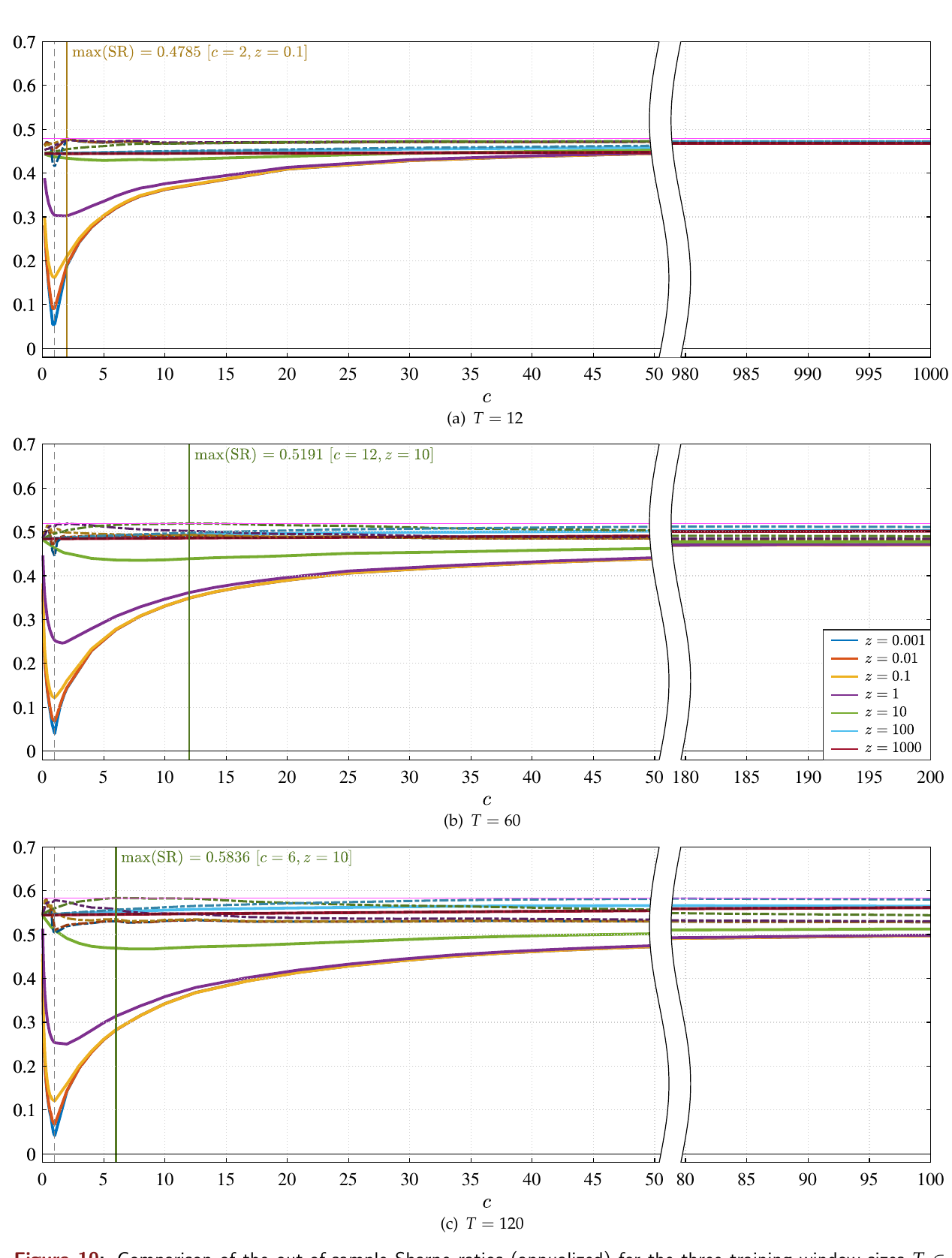
The monotone concave shape is gone even under the per-draw averaging. The curves now start high, sag toward a trough at the interpolation boundary where c equals 1, then recover. Adding random features to a simple model makes it worse up to that boundary, which is the opposite of the advertised result. Maximum Sharpe ratios land at complexity 2, 12 and 6 for the three training windows, not at 1000.

One more detail closes the loop. With an intercept, the simplest possible random-feature model, P equals 2, at heavy shrinkage reproduces the rolling historic average forecast to four decimal places: 0.4443, 0.4842 and 0.5446 for the three windows. The intercept-only model was always there. The zero restriction was hiding it.

The machine did not learn to be long-only

Kelly, Malamud and Zhou also claim their complex model discovers the Campbell-Thompson positivity constraint on its own, calling the high-complexity strategy "long-only at heart" and noting that the machine appears to learn the rule without being told. Their evidence is the asymmetry of the timing weights.

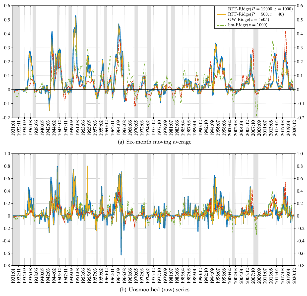
The weights do skew positive. They also skew positive for the 500-feature model, for a 15-predictor ridge regression at heavy shrinkage, and for a univariate regression on book-to-market alone. Any model fit through the origin on a target with a positive mean produces this. The correlation between the complex model's weights and the 500-feature model's weights is 0.9987.

Let the intercept float and the asymmetry vanishes for every model at once.

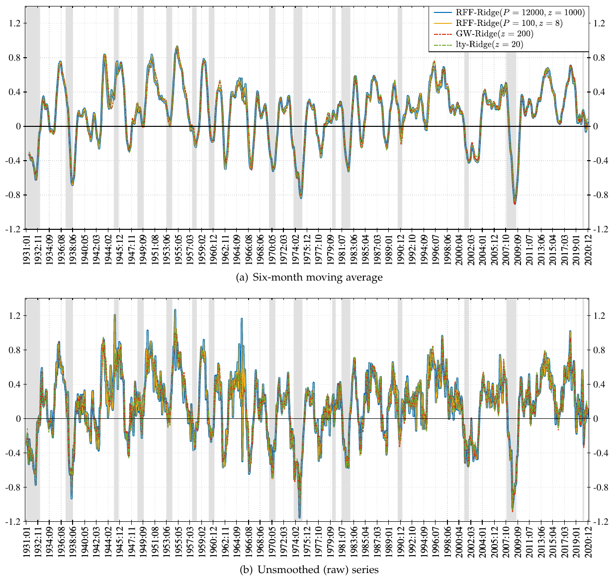
Four lines, one visible series. The correlation between the 12,000-feature model and a 100-feature model rises to 0.9999. Against a univariate ridge regression on long-term yield alone it is 0.9661. The complex model and a single-variable regression are producing the same positions. And since these forecasts come from rolling 12-month windows, they are time-varying weighted moving averages of the last 12 monthly returns, which is enough on its own to reproduce the celebrated behaviour of divesting ahead of recessions. Buncic quotes Samuelson on the market having predicted nine of the last five recessions, which is the right response.

What actually wins, and why you should not buy that either

Over the common January 1940 to December 2020 window, the ranking runs: expanding-window ridge on the 15 Goyal-Welch predictors with mild shrinkage at 0.6990, rolling-window ridge on the same 15 at 0.6127, a univariate regression on the term spread at 0.6789, buy-and-hold at 0.5494, the rolling 120-month historic average at 0.5446, the best random-feature model at 0.5863, and the headline complex model at 0.4851. Expected returns tell the same story: 0.044 for the complex model at T equals 120 against 0.859 for the best expanding-window linear model, a factor of roughly 20.

This is where I part company with the paper's framing. Those 0.699 and 0.6127 figures are grid maxima. Buncic searches roughly 40 shrinkage values, crossed with rolling and expanding windows and three training window sizes, and reports the best, evaluated on the same 1940 to 2020 sample used to pick it. The 0.4851 he compares them against is a single pre-specified configuration. Comparing a maximum over a few hundred configurations to a point estimate is the selection bias that the old article "Parameter Stability Beats Best Parameter" spends its length warning about, and the paper reports no deflated or selection-adjusted number. The honest version of the comparison is narrower: with an intercept, simple models are competitive with the complex one and the ordering in complexity reverses. Whether a 15-predictor ridge regression beats buy-and-hold out of sample by 0.15 of a Sharpe ratio is a separate question this paper does not settle.

Two other cracks are worth naming. The predictor set uses contemporaneous inflation, which posts about two weeks into the following month, so every model here carries a look-ahead. Buncic reruns with lagged inflation and reports that random-feature Sharpe ratios drop across the board for all P and z, which means the complex models were leaning on the leak harder than the simple ones. And nothing in the exercise charges a cost. A strategy that re-sizes its position every month off a 12-observation refit turns over constantly, and the pooled random-feature portfolio is an average of 1,000 books.

The generalizable lesson is not that complexity fails. It is that a theoretical result about complexity got confirmed by an empirical design where two settings unrelated to complexity, an origin restriction and a scoring convention, controlled the entire shape of the answer. The old article "Why Simplicity Is a Statistical Weapon" makes the case for small models on variance grounds. This is a different and more uncomfortable case: the measurement apparatus produced the result. Before you believe any curve that rises with a knob, turn the other knobs and check that the curve is still there. The old article "Does ML Actually Help Asset Pricing? Kelly's 20%, Not 2–3×" reaches the same destination from the returns side.

KEY POINTS

• KMZ's stated 0.47 annual Sharpe ratio improvement over buy-and-hold is not an improvement. Buy-and-hold earns 0.5494 on the same standardized series over the common January 1940 to December 2020 window, and their headline 12,000-feature model earns 0.4851.
• The zero-intercept restriction is doing the work. The target has a mean of 0.1590 with a t-statistic of 4.47, so forcing the fit through the origin makes the slopes manufacture the mean. Squared bias falls from 0.0130 to 0.0267 down to under 0.0002 once the intercept floats and stays out of the ridge penalty.
• Allow an intercept and the complexity ordering reverses. Best random-feature Sharpe ratios go 0.4745, 0.5157, 0.5863 for training windows of 12, 60 and 120 months. Longer window means lower complexity, since c equals P over T, so performance improves as complexity falls.
• The VoC curve comes from scoring 1,000 random draws separately and averaging the scores, while KMZ's own Table I averages the forecasts first. A single draw with P features self-averages P/2 feature pairs, so per-draw noise shrinks like one over the square root of P. A simulated strategy with a fixed true Sharpe ratio of 0.45 traces the same monotone concave curve from 0.03 to 0.44 under that scoring rule.
• Watch for the impossible number: at P equals 2 and T equals 120 the per-draw averaging returns Sharpe ratios near minus 0.0017 alongside positive expected returns and positive alphas. A real portfolio cannot do that. An average of ratios can.
• The "machine learns to be long-only" claim is the same restriction seen twice. Free the intercept and the timing weights from a 12,000-feature model correlate 0.9999 with a 100-feature model and 0.9661 with a single regression on long-term yield.
• Do not swap one grid maximum for another. The 0.6990 and 0.6127 linear results are the best of roughly 40 shrinkage values crossed with two window types and three window sizes, scored on the sample used to select them, with no deflation reported. Add contemporaneous inflation in the predictor set, which posts two weeks late, and zero transaction costs on a monthly-rebalanced book, and treat every number here as gross.

References

• The Virtue of Complexity in Return Prediction (Kelly, Malamud, Zhou, 2024)
• A Comprehensive Look at the Empirical Performance of Equity Premium Prediction (Goyal, Welch, 2008)
• Predicting Excess Stock Returns Out of Sample: Can Anything Beat the Historical Average? (Campbell, Thompson, 2008)
• A Comprehensive 2022 Look at the Empirical Performance of Equity Premium Prediction (Goyal, Welch, Zafiropoulos, 2024)
• Empirical Asset Pricing via Machine Learning (Gu, Kelly, Xiu, 2020)
• Comment on 'The Virtue of Complexity in Return Prediction' (Berk, 2023)
• Simplified: A Closer Look at the Virtue of Complexity in Return Prediction (Daniel Buncic, 2025)

A note on AI. The ideas, research, analysis, and conclusions in this article are my own. I use AI tools to help with editing and wordsmithing, because English is not my first language, and I am not shy about that. AI-generated ideas and AI-assisted writing are not the same thing: the first is empty slop from a generic prompt, the second is a tool for communicating years of real research more clearly. Judge the work by its substance, not by whether software helped polish the prose.