7.5 The Mathematics of Machine Learning, for Traders

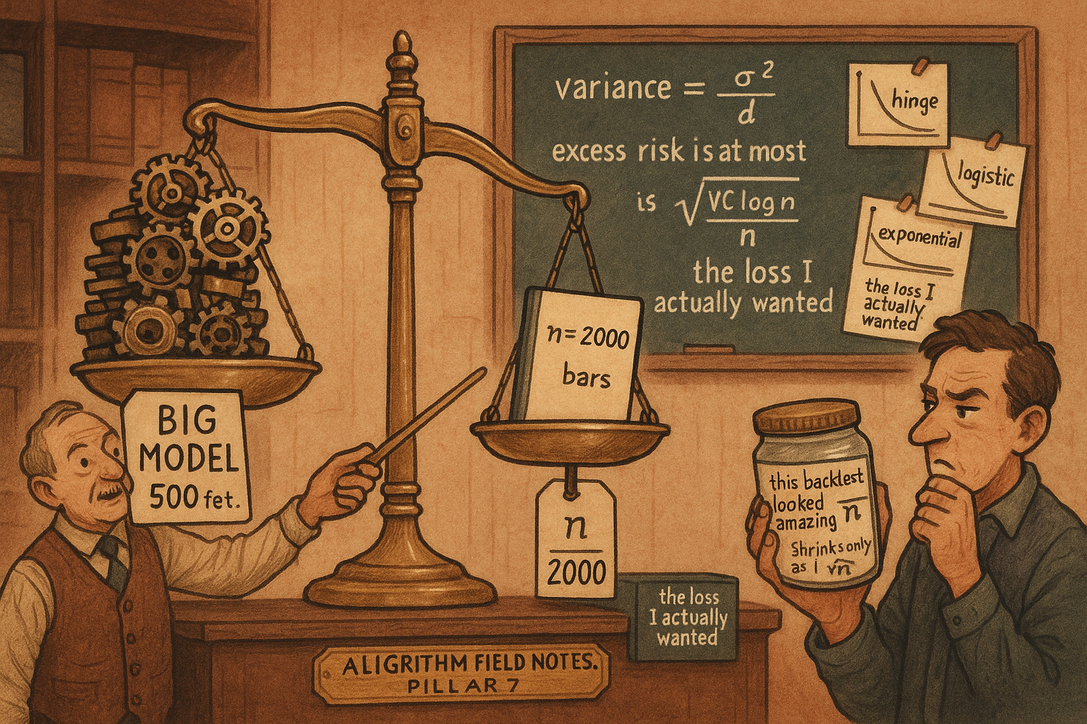
You already ran the models. The old article "From One Tree to Forests to Boosting" walked you from a single decision tree to XGBoost, "How a Decision Tree Engineers a New Alpha" showed a tree carving conditional edges out of order-book features, and "Ridge Above 1h, XGBoost Below 5min" handed you a timeframe rule for which model to point at which horizon. None of those articles answered the one question that decides whether any of it survives contact with next month's data: why should a function fit on the past predict the future at all? Nothing in the arithmetic of a backtest forces that to be true. The math of machine learning is the part that tells you when it is, and by how much, and what you pay for reaching for a bigger model.

This is the theory sitting under the whole ML arc. It is not decoration. Every skeptical instinct the robustness articles kept repeating, that complexity is expensive, that in-sample fit is a liar, that more parameters means more variance, turns out to be a theorem with a rate attached. Once you see the rate you stop arguing about it.

The best you can possibly do, and why you never reach it

Start with the target. You have an input X (your features) and an output Y (next return, or its sign). You pick a function h to predict Y from X, and you grade it with a loss. For a sign classifier the natural loss is misclassification: zero when you call the direction right, one when you call it wrong. The risk is the expected loss over the true, unknown distribution of the market.

The function that minimizes that risk is not mysterious. In the sign-prediction case it is the Bayes classifier, and it depends on one quantity, eta of x, the probability that Y equals plus one given the features equal x.

$$ \eta(x) := \mathbb{P}(Y = 1 \mid X = x), \qquad h_0(x) = \begin{cases} +1 & \text{if } \eta(x) > 1/2 \\ -1 & \text{otherwise.} \end{cases} $$

Read it plainly. If the features say the odds of an up-move are better than even, bet up. Otherwise bet down. That is the best classifier that exists, and its error rate is the Bayes risk, the floor no model beats.

Work a number. Say for one feature bucket the true up-probability eta is 0.58. The Bayes rule bets up and is wrong 42% of the time. That 42% is irreducible, market noise that no feature removes. A trader who expects a direction model to hit 90% on liquid futures is asking to beat the Bayes risk, which is impossible. The realistic question is never "can I hit the floor," it is "how far above the floor does my model sit, and is that gap worth trading."

You never reach the floor for a blunt reason: you do not know eta of x. You have a finite sample, and you minimize the loss you can compute, the training error, over some class of candidate functions. That substitution, true risk replaced by average training loss, is empirical risk minimization, and it is what every fit you have ever run actually does.

Every parameter costs you sigma-squared over n

Here is the first theorem with real teeth for a trader. Fit ordinary least squares with d basis functions (d features, or d columns of a polynomial expansion) on n data points, where the noise variance is sigma-squared. Decompose the expected prediction error and the variance you added by estimating d coefficients comes out exactly:

$$ \mathbb{E}R(\hat h_D) \;=\; \underbrace{\text{squared bias}}_{\text{falls as } d \uparrow} \;+\; \underbrace{\frac{\sigma^2 d}{n}}_{\text{variance}} \;+\; \underbrace{\mathbb{E}\,\mathrm{Var}(Y\mid X)}_{\text{irreducible}}. $$

The middle term is the price of complexity, and it is linear in d. Every parameter you add pours another sigma-squared over n of variance into your out-of-sample error, whether or not that parameter helps. Bias falls when you add useful features; variance rises no matter what.

Put numbers on it. Take sigma-squared equal to 1 and n equal to 200 bars. A five-parameter model carries variance 5 over 200, which is 0.025. Push to forty parameters and variance becomes 40 over 200, which is 0.20. You bought 35 extra coefficients and paid 0.175 in guaranteed out-of-sample error, and they only earn their keep if they cut squared bias by more than that. On 200 bars they almost never do.

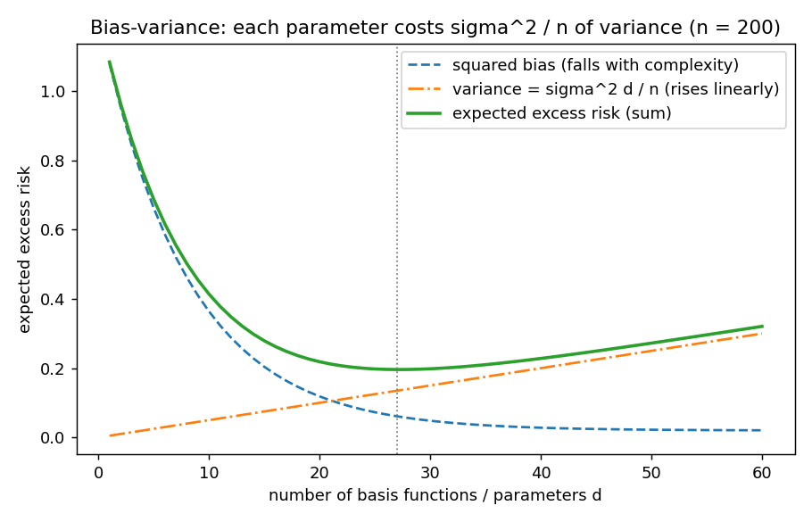
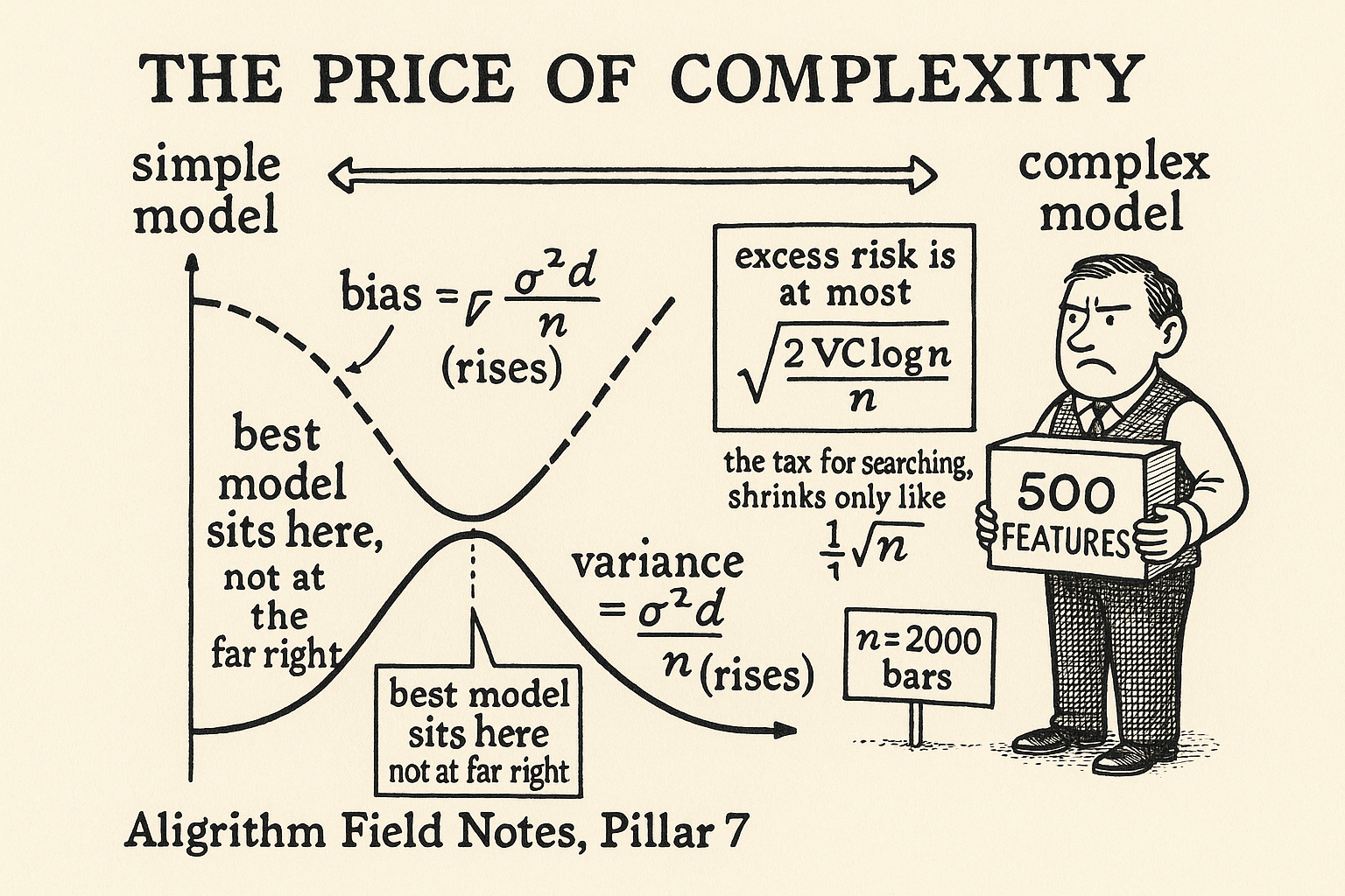
The curve is U-shaped and the minimum sits well short of the richest model your software will let you fit. This is the exact mechanism behind the old article "The Limits of Linear Models" and the reason "Regularization from First Principles" exists: shrinkage deliberately biases the coefficients toward zero to buy back some of that sigma-squared d over n. The trade is more bias for less variance, and on short, noisy financial samples it usually wins. The math here is why.

Cross-validation estimates the wrong thing, on purpose

You cannot see the true risk, so you estimate it. v-fold cross-validation splits the data into v blocks, trains on v minus one of them, scores on the held-out block, and rotates.

$$ \mathrm{CV}(j) := \frac{1}{n} \sum_{k=1}^{v} \sum_{i \in A_k} \ell\!\left( \hat h_{-k}^{(j)}(X_i),\, Y_i \right). $$

The honest caveat the notes make explicit: this is a biased estimate. Each fold trains on only a fraction of the data, so cross-validation reports the error of a model fit on n times (v minus one) over v points, not on all n. Run 5-fold on 500 bars and every model is scored while trained on 400 bars, then rotated across the five held-out blocks of 100. The number you read off is the error of a 400-bar model, and it is pessimistic for the 500-bar model you will actually deploy. Leave-one-out (v equal to n) has the least bias but the folds overlap almost completely, so the scores are highly correlated and the estimate is noisy. Typical choice is v equal to 5 or 10, a deliberate compromise between bias and variance of the estimate itself.

For a trader this maps onto a familiar pitfall. Cross-validation on shuffled financial data leaks the future into the training folds through autocorrelation, so the CV number flatters the model. The purged, embargoed splits the robustness articles push are the same v-fold idea with the leakage plugged. The estimator is only as good as the independence of its folds, and market data violates independence by construction.

Trees are unstable, and averaging has a floor

A single regression tree splits the feature space greedily to cut residual sum of squares, then predicts the mean response in each leaf. The old article "How a Decision Tree Engineers a New Alpha" covered that machinery. The theory adds the warning: the greedy build is unstable, so a small change in the training data flips an early split and hands you a different tree. High variance, in the exact sense of the decomposition above.

Random forests attack that variance by averaging B trees grown on bootstrap resamples, each split restricted to a random subset of features. The reason the feature sampling matters falls straight out of the variance of an average of correlated things:

$$ \mathrm{Var}\big(f_{\text{rf}}(x)\big) = \frac{1-\rho}{B}\,\mathrm{Var}\big(\hat T^{(1)}(x)\big) \;+\; \rho\,\mathrm{Var}\big(\hat T^{(1)}(x)\big). $$

Rho is the correlation between two trees' predictions. The first term shrinks to nothing as you grow more trees. The second term does not depend on B at all. Grow ten thousand trees and the variance still cannot fall below rho times a single tree's variance.

Numbers. Let a single tree's variance be 1 and let the trees correlate at rho equal to 0.3. With B equal to 100 trees the forest variance is 0.7 over 100 plus 0.3, which is 0.307. With B infinite it is still 0.30. Adding trees past a point is free of benefit; the floor is set by rho. That is why the algorithm samples features at each split: it forces the trees apart, dropping rho toward 0.05, which drops the floor to 0.05. The whole point of a random forest is not the bagging, it is the decorrelation.

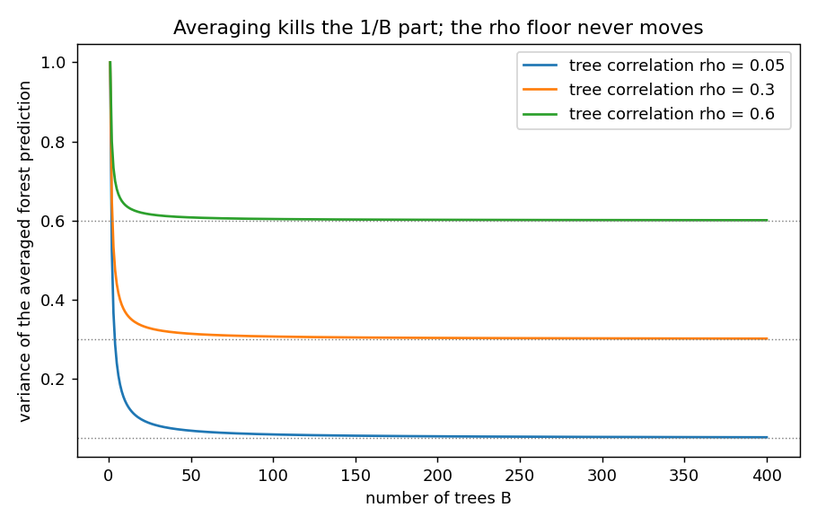
For a trader this is the quantitative version of "your ensemble members are too similar." Ten models built on the same features with the same target are one model wearing ten hats, and no amount of averaging escapes their shared variance.

The price of complexity, as a bound you can compute

Now the centerpiece. How far can training error drift from true error across a whole class of candidate models? For a finite class of size the-cardinality-of-H, Hoeffding's inequality plus a union bound gives, with probability at least 1 minus delta:

$$ R(\hat h) - R(h^*) \;\leq\; \sqrt{\frac{2\big(\log|\mathcal{H}| + \log(1/\delta)\big)}{n}}. $$

The left side is excess risk, how much worse your fitted model is than the best model in the class. The right side is the tax you pay for searching. It grows with the log of how many models you tried and shrinks like one over the square root of the sample.

Worked example. You grid-search 1000 candidate configurations, n equal to 500 bars, delta equal to 0.05. The bound is the square root of 2 times (log 1000 plus log 20) over 500, which is the square root of 2 times (6.91 plus 3.00) over 500, which is the square root of 0.0396, about 0.20. Your out-of-sample error could sit a full 20 percentage points above the best-in-class model purely from the search. Push n to 50,000 and the same bound falls to about 0.02. Sample size is the only thing that buys the tax down, and it buys slowly.

Infinite model classes (linear models over a continuum of coefficients, all trees) need a finer tool than counting. The count gets replaced by the VC dimension, the largest number of points the class can label in all possible ways. The Sauer-Shelah lemma says a class of VC dimension d can only produce polynomially many labelings, (n plus 1) to the d, instead of the two-to-the-n a truly unrestricted class would, and that collapses the bound to:

$$ \mathcal{R}_n(\mathcal{F}) \;\leq\; \sqrt{\frac{2\,\mathrm{VC}(\mathcal{H})\,\log(n+1)}{n}}. $$

The useful fact for a trader: for linear classifiers on p features, the VC dimension is exactly p, bounded above by the dimension of the underlying function space. So a linear sign model on 10 features, with n equal to 1000, carries an excess-risk bound near the square root of 20 times log(1001) over 1000, about 0.37. At n equal to 100,000 it drops to about 0.05. The dimension of your feature set enters the guarantee directly, and it enters through a one-over-root-n rate that no clever fit accelerates. A tree over the same features has a much larger VC dimension, which is one more reason the old article "Linear Models' Hidden Symmetry Advantage" preferred the linear form for short-horizon sign models: fewer effective degrees of freedom, a tighter bound, and the buy-sell symmetry built in for free.

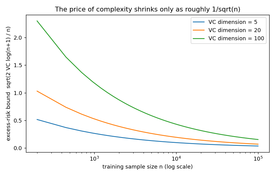
This is the theorem behind every warning about degrees of freedom. More candidate models, more features, richer class, all push the bound up, and the only counterweight is more genuinely independent data. On a strategy with 2000 non-overlapping bars, the bound is loose enough that a large model's in-sample edge tells you almost nothing.

Why you never optimize the loss you actually care about

Misclassification loss is a step function, flat then a cliff at zero. Minimizing it over linear models is not convex and not even continuous, so it is computationally hopeless. The fix that makes machine learning tractable is to replace the 0-1 loss with a convex surrogate that hugs it from above.

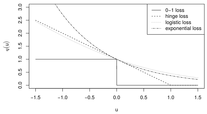
The three that run the field are hinge loss (max of 1 minus u and 0, the support vector machine), exponential loss (e to the minus u, the engine of AdaBoost), and logistic loss (log of 1 plus e to the minus u, logistic regression), where u is the margin y times h of x, positive when you are right.

$$ \phi_{\text{hinge}}(u) = \max(1-u,\,0), \qquad \phi_{\text{exp}}(u) = e^{-u}, \qquad \phi_{\text{log}}(u) = \log_2\!\big(1 + e^{-u}\big). $$

Put a margin through them. At a correct-but-marginal call, u equal to 0.5, hinge charges 0.5, logistic charges log-base-2 of 1 plus e-to-the-minus-0.5, about 0.66, and exponential charges e-to-the-minus-0.5, about 0.61. At a confident miss, u equal to minus 1, exponential explodes to e, about 2.72, while hinge charges only 2 and logistic about 1.88. Exponential loss punishes bad misses hardest, which is why AdaBoost chases outliers so aggressively and why a few mislabeled bars can dominate its fit.

The reason this substitution is legitimate, not a hack, is classification calibration: a convex surrogate whose derivative at zero is negative drives its minimizer to the same sign as the Bayes classifier. All three above qualify. You optimize a smooth convex proxy, and you still recover the right decision boundary. That single result is why gradient-based training works and why your logistic regression and your SVM are chasing the same target through different smooth approximations of a cliff.

Sparsity is a bet, and the math prices it

Constraining the coefficient norm controls the class complexity, and the choice of norm decides how the guarantee scales with the number of features p. Bounding the L2 norm (ridge) gives an excess-risk rate of order the square root of p over n. Bounding the L1 norm (lasso) gives order the square root of s log p over n, where s is the number of features that actually matter.

$$ \ell_2:\quad \sqrt{\frac{p}{n}} \qquad\qquad \ell_1:\quad \sqrt{\frac{s\,\log p}{n}}. $$

Worked case. You have p equal to 1000 candidate features, but suspect only s equal to 10 carry signal, on n equal to 2000 bars. The L2 rate is the square root of 1000 over 2000, about 0.71. The L1 rate is the square root of 10 times log 1000 over 2000, about 0.19. When the truth is sparse, L1 trades a factor of p for a factor of s log p and wins by a mile. When every feature matters equally, the two rates converge and L2 is the cleaner choice. This is the formal statement of what "Regularization from First Principles" argued by intuition: lasso is a bet that most of your features are noise, and the bet pays only when it is true.

Gradient descent converges at one over root k, and stochastic descent matches it

Fitting these convex objectives means minimizing a convex function, often non-differentiable (hinge loss has a kink). Subgradients handle the kink: any supporting line below the function counts as a gradient, and gradient descent steps against it, projecting back onto the constraint set each step. The convergence guarantee is clean:

$$ f(\bar\beta) - f(\hat\beta) \;\leq\; \frac{2LR}{\sqrt{k}}, $$

where k is the number of iterations, R bounds the size of the feasible set, and L bounds the subgradient norm. Error falls like one over the square root of the step count. To get within 0.02 of the optimum with L and R both equal to 1 you need about 10,000 iterations, since 2 over the square root of 10,000 is 0.02.

The move that makes this scale to real data is stochastic gradient descent. Computing the full gradient sweeps all n points every step. SGD replaces the full gradient with the gradient at a single randomly drawn point, and the expected-error bound is identical, 2LR over root k. You pay nothing in the rate for using one sample at a time instead of all n, which is why SGD trains models on datasets too large to hold a full gradient for. The catch the notes are honest about: this rate is for convex objectives, and a neural network is wildly non-convex, so the guarantee does not transfer. SGD works on deep nets empirically, not because a theorem promises it.

Boosting and backprop, in one breath each

AdaBoost is greedy empirical risk minimization on the exponential loss. Each round it fits a weak classifier to reweighted data and adds it with weight:

$$ \hat\beta_m = \frac{1}{2}\,\log\!\left(\frac{1 - \operatorname{err}_m}{\operatorname{err}_m}\right), $$

where err-sub-m is the weighted error of that round's weak learner. A learner with error 0.4 gets weight one-half log of 0.6 over 0.4, which is 0.20. A sharper learner with error 0.1 gets one-half log of 9, which is 1.10. Better weak classifiers earn exponentially more say, and misclassified points get upweighted so the next round focuses on them.

Gradient boosting drops the exponential-loss specialization and treats the whole thing as gradient descent in function space: fit each new tree to the negative gradient of the loss at the current predictions. For squared error that gradient is proportional to the residual, so gradient boosting is repeatedly fitting a tree to what the current model got wrong, then adding a shrunk version of it. That is the literal mechanism inside the LightGBM and XGBoost the old article "From One Tree to Forests to Boosting" told you to use below five minutes.

Backpropagation is the chain rule applied to the layered composition of a feedforward network, computing the gradient of the loss with respect to every weight in one backward sweep. Forward pass to get the activations, backward pass to accumulate derivatives layer by layer. It is fast because the compositional structure lets each layer reuse the derivative computed by the layer above it, and it is the only reason training a deep network is feasible at all.

Where this lands for a trader

None of this tells you which features carry alpha. It tells you the exchange rate between complexity and data, and that rate is unforgiving. Excess risk falls like one over the square root of n, so quadrupling your sample halves your guarantee. Complexity, measured by parameter count or VC dimension, enters that guarantee directly and multiplies the tax. Variance from estimating coefficients is sigma-squared d over n whether the coefficients help or not. Averaging correlated models hits a floor set by their correlation, not by how many you stack.

Every one of those is a theorem, not an opinion, and every one of them says the same thing the empirical robustness work has been saying: on short, noisy, dependent financial data, the small model with the honest out-of-sample test beats the big model with the pretty backtest, and the reason is arithmetic. The old article "QLike: The Right Loss Function for Vol Forecasting" made the point that the loss you optimize is a modeling choice with money attached; the surrogate-loss and calibration results here are the same point one level down, about the loss you can actually compute versus the one you care about. Pick the model your sample size can afford, and let the rate decide, not the fit.

KEY POINTS

• The Bayes classifier bets on whichever sign has probability above one-half, and its error rate is the irreducible floor. No model beats it, so a direction model hitting 90% on liquid futures is a red flag, not a triumph.
• Empirical risk minimization substitutes average training loss for the true risk you cannot see. Every fit you run does this, and the gap between the two is the whole subject.
• Each estimated parameter adds sigma-squared over n of variance to out-of-sample error, useful or not. Variance is linear in the number of parameters d; bias only falls if the parameter helps. This is why the optimal model is U-shaped short of the biggest one you can fit.
• Cross-validation is a deliberately biased estimate that scores a model trained on a fraction of the data. On autocorrelated financial data the folds leak the future unless you purge and embargo, which is why the CV number flatters bad models.
• A random forest's variance cannot fall below the tree-to-tree correlation rho times a single tree's variance, no matter how many trees you grow. The feature sampling exists to push rho down, not to add trees.
• Excess risk is bounded by roughly the square root of (VC dimension times log n over n). More candidate models, more features, and richer classes all raise the tax; only more independent data lowers it, and it lowers like one over root n.
• You never minimize misclassification loss directly; you minimize a convex surrogate (hinge, logistic, exponential) that is classification-calibrated, meaning its minimizer has the right sign. This is why gradient training works at all.
• L1 (lasso) beats L2 (ridge) at a rate of square-root s-log-p over n versus square-root p over n, but only when the truth is sparse. Sparsity is a bet the math prices explicitly.
• Gradient descent and stochastic gradient descent both converge like 2LR over root k on convex objectives, so using one data point at a time costs nothing in the rate. The guarantee does not extend to non-convex nets.
• Gradient boosting fits each new tree to the current residual; AdaBoost weights each weak learner by one-half log of (1 minus error) over error; backprop is the chain rule in one backward sweep. All three are the machinery under the models the ML arc told you to run.

References

• Statistically Sound Indicators for Financial Market Prediction - Timothy Masters (Amazon)
• Systematic Trading - Robert Carver (Amazon)
• Mathematics of Machine Learning (maths of ML)