2. Indicator Engineering June 28, 2026 5 min

2.79 How a Decision Tree Engineers a New Alpha

A decision tree mines conditional alphas by carving feature space into boxes. It picks each split to maximize a similarity gain and predicts the mean return per leaf. Stop early or it memorizes noise.

The old article "The Limits of Linear Models" ended on a rule instead of an equation: if realized vol is high and the trend is weak, fade momentum and lean mean-reversion. That rule is a decision tree with one split. This article builds the machine that finds rules like it on its own, because hand-writing them does not scale. You have momentum, value, realized vol, dispersion, trend strength, and a dozen more, and the conditional combinations run into the thousands. You need a procedure that mines the conditions for you.

Start with the training data. Each row is a moment in time: the values of every signal at that instant, paired with the future return that followed. The target is the future return, the features are the cross-sectional signals, and you have millions of rows. The job is to carve this data into regions where the future return behaves the same way inside each region.

The split is a question that sorts the data

A tree asks one yes-or-no question and splits the rows into two groups by the answer.

realized_vol > 80th pct ?
momentum < 0 ?

Each question puts some rows on the left and the rest on the right. A good question puts rows with similar future returns together: outperformers on one side, underperformers on the other. A useless question scatters them evenly across both sides, so neither group tells you anything. The whole game is finding the question that separates best, then repeating it on each of the two groups, and again on their children, until you stop.

This is the same instinct as fitting a linear regression, where you pick the line that minimizes squared error. A tree picks the split that minimizes squared error too, just within the groups instead of along a line. The standard CART formulation writes this as maximizing a similarity gain, which is the same arithmetic seen from the other side, and it is worth writing out because the formula is the entire engine.

The similarity score and the gain

Score a group of rows by how spread out their future returns are. Take each row's return, subtract the group's mean return, square the difference, sum across the rows, and divide by the count.

$$ \text{similarity(node)} = \frac{\sum_{i \in \text{node}} \big(y_i - \bar{y}\big)^2}{n_{\text{node}}} $$

A low score means the returns in that group sit tight around their mean, so the group is internally consistent and its mean is a confident prediction. A high score means the returns are all over the place and the mean tells you little. You want splits that drive this score down in the children.

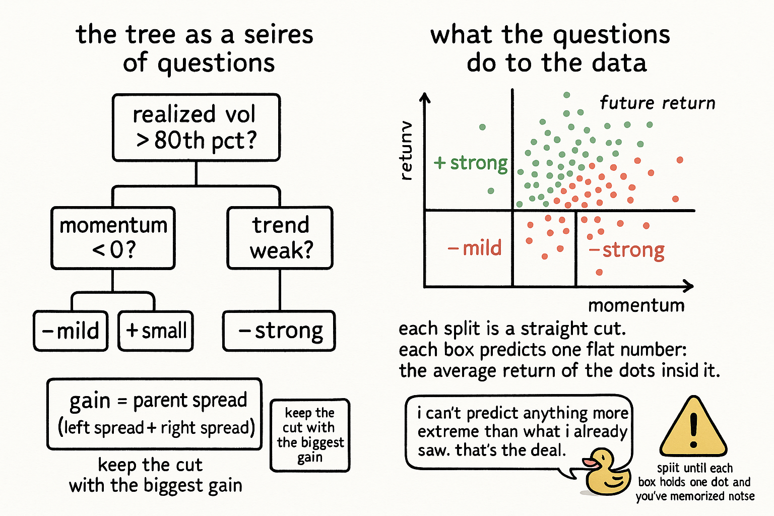
Measure that with the gain: the parent's score minus the sum of the two children's scores.

$$ \text{gain} = \text{similarity(parent)} - \big(\text{similarity(left)} + \text{similarity(right)}\big) $$

To pick the split at a node, the tree scans every feature and every candidate threshold on that feature, computes the gain for each, and keeps the one with the largest gain. "Momentum below zero" wins if cutting the data there leaves outperformers piled on one side and underperformers on the other better than any other cut. Then the procedure recurses: each child node runs the same scan on its own rows and finds its own best split, building the tree one question at a time.

The prediction is a flat number per region

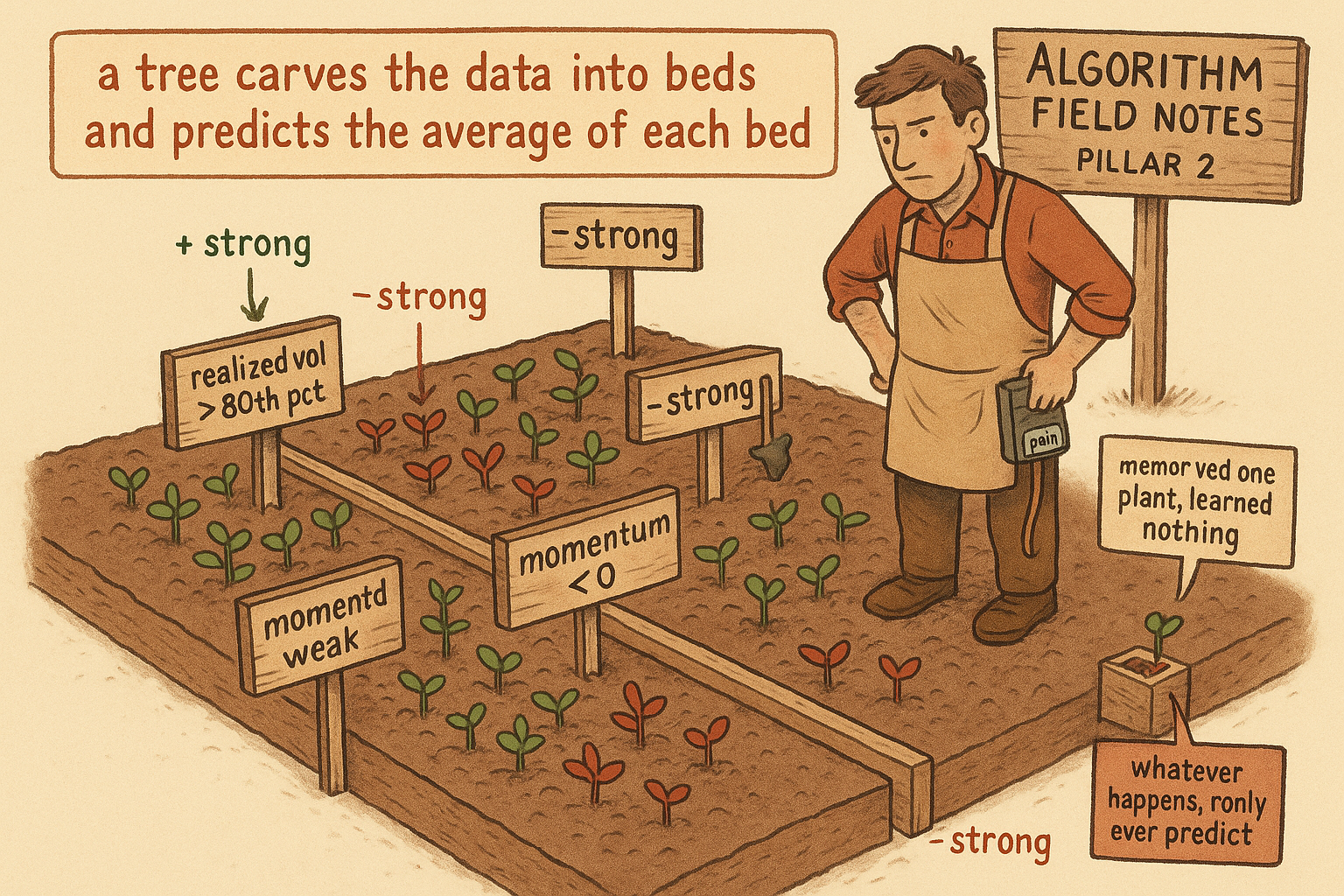
When a node stops splitting, it becomes a leaf, and the leaf predicts the mean future return of the rows that landed in it.

$$ \text{prediction(leaf)} = \bar{y}_{\text{leaf}} = \frac{1}{n_{\text{leaf}}} \sum_{i \in \text{leaf}} y_i $$

Trace a new market state down the tree, answering each question, and you land in one leaf and read off its mean. That number is the forecast. Notice what the tree has built: it has carved the feature space into boxes, and inside each box it predicts a single constant. "When realized vol is high and the trend is weak and momentum is negative, the next return averages slightly negative" is one box. The tree discovered that conjunction by splitting, which is the interaction the linear model could not represent. This is the sense in which a tree engineers a new alpha. It manufactures conditional signals out of raw features by finding the conditions where the raw features mean something.

Three problems this opens, on purpose

The construction is simple, and the simplicity hides three questions that decide whether the tree makes money or fits noise.

When do you stop splitting? Keep splitting and you can drive every leaf down to a single row, where the similarity score is zero and the prediction is that one row's return. That tree has memorized the training data and learned nothing, the textbook overfit. You stop early, with a minimum number of rows per leaf or a maximum depth or a minimum gain to bother splitting, and where you set those knobs is the same plateau-versus-peak choice the old article "Parameter Stability Beats Best Parameter" makes for any parameter. The old article "How to Test Indicator Thresholds Without Fooling Yourself" applies directly too, because a tree's split search is a threshold search run thousands of times, and an unconstrained one finds thresholds that work in-sample and die out.

Why are the predictions discrete and bounded? A leaf predicts an average of training returns, so the tree can only ever output one of a finite set of leaf means, and none of them can exceed the most extreme average it saw. A linear model extrapolates past its training range; a tree cannot. Hand it a state more extreme than anything in the data and it returns the nearest leaf's tame average, which caps the upside and the downside of the forecast.

How do you stop one tree from being fragile? A single tree's early splits are chosen from noisy data, and a small change in the sample can flip the top split and rebuild the whole tree differently. That instability is the subject of the next step in this arc, "From One Tree to Forests to Boosting," which trades one fragile tree for many and gets a stable forecast back. The long-short symmetry a single tree breaks, the subject of "Linear Models' Hidden Symmetry Advantage," has to be engineered back here too, because each split learns its threshold from one side of the mirror.

Visualizing the carve

KEY POINTS

A decision tree carves the training data into regions by asking yes-or-no questions on features, so that future returns inside each region behave alike. Each question is a split like "momentum below zero?".
Score a group by how tightly its returns cluster around their mean: the summed squared deviations divided by the count. Low score means a confident prediction, high score means the mean tells you little.
Pick the split with the largest gain, the parent's score minus the two children's scores. The tree scans every feature and threshold, keeps the best cut, then recurses on each child.
A leaf predicts the mean future return of the rows in it. The tree carves feature space into boxes and predicts a constant per box, which is the interaction a linear model could not represent. That is how a tree engineers a conditional alpha.
Stopping is the overfitting control. Split all the way and every leaf memorizes one row. Stop early with minimum leaf size, max depth, or a minimum gain, and choose those knobs on a stable plateau, not an in-sample peak.
Tree predictions are discrete and bounded: only leaf means, none more extreme than the most extreme average seen. A tree does not extrapolate. A single tree is also fragile, which the move to forests and boosting fixes.