2.80 Ridge Above 1h, XGBoost Below 5min
Pick the model by interaction strength: ridge when near-additive, XGBoost when interactions dominate. XGBoost also handles NaNs natively, avoiding imputation lookahead; else use an IC-weighted ensemble.
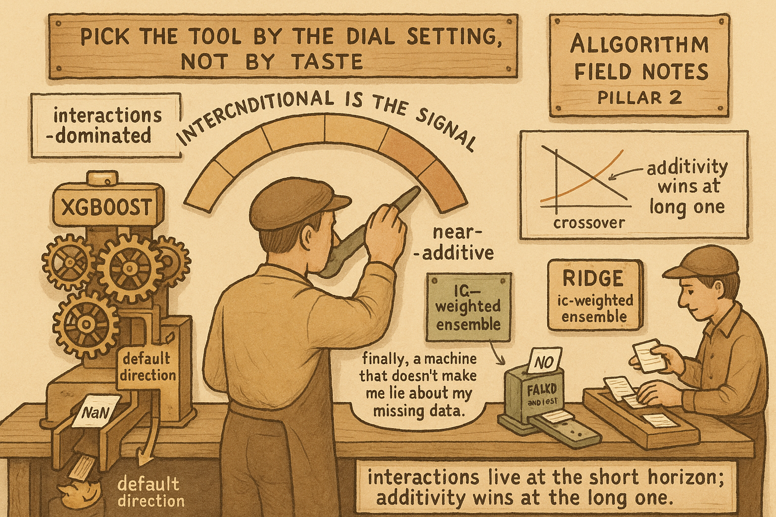
Pick the model by how strong the interactions are, not by fashion. At longer, near-additive horizons, ridge regression is the right tool. At shorter, interaction-dominated horizons, gradient-boosted trees win, and they win by enough to matter. The crossover is not a fixed clock time you read off a tweet; it is the horizon where the conditional structure starts to dominate the additive structure, and which side of it you are on should decide your model before you tune a single hyperparameter.
The reason is the same conditional structure the rest of this arc has been circling. The old article "The Limits of Linear Models" showed that signal relationships are interactions: momentum pays in low-vol clean-trend regimes, carry crashes when vol spikes. Those interactions are strongest at the shortest horizons, where the next move depends on the regime you are sitting in. As you stretch the horizon out, the regime conditioning washes out, the surviving signal flattens into something close to additive, and a regularized linear model captures it with less variance than a tree ever could.
The thing that decides it
Score the forecasts with the information coefficient, the correlation between the forecast and the realized return. It is the standard yardstick because it survives the near-zero signal-to-noise the old article "Why Volatility Is More Non-Stationary Than Trend" describes: you are not trying to nail the return, you are trying to be correlated with it across many predictions.
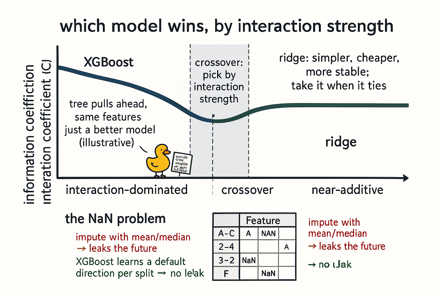
Where the signal is near-additive, ridge and a tuned XGBoost land in roughly the same place on IC, so you take the simpler, cheaper, more stable model. Where interactions dominate, the tree pulls meaningfully ahead, and it needs careful tuning to do it. The point is not a precise IC delta you can quote; it is the direction of the gap.
$$ \text{IC}_{\text{tree}} > \text{IC}_{\text{ridge}} \;\;\text{(interactions dominate)} \qquad \text{IC}_{\text{tree}} \approx \text{IC}_{\text{ridge}} \;\;\text{(near-additive)} $$
The edge, when it shows up, is paid purely for using a better model on the same features. Call it a few IC points if you need an illustrative figure, but treat that as a stand-in, not a promise; the real number depends on your features and horizon. The tree is not seeing different data. It is extracting the interactions out of the same columns that ridge has to treat additively, and at the horizon where interactions dominate, that extraction is the whole game.
XGBoost eats NaNs, and that is not cosmetic
The second reason to reach for XGBoost at short horizons has nothing to do with accuracy on clean data. It handles missing values natively, and missing values are the normal state of a real feature set.
Your features come from different sources with different histories. One data provider has ten years of a given feed, another has two. One exchange feed has a gap. A feature with a long lookback is undefined for the first part of any window. So at any given row, some features are present and some are NaN, and which ones are missing changes over time. A linear model cannot multiply a weight by a NaN. You are forced to do something about the holes before the model runs.
The obvious move is imputation: fill each NaN with the feature's mean or median. That move has a subtle lookahead the old article "How to Test Indicator Thresholds Without Fooling Yourself" would flag on sight. The mean or median is computed over data that includes the future relative to the row you are filling, so you are leaking the feature's future distribution into a past prediction. You can compute a lookahead-free running mean instead, expanding-window only, and it is better, and it still bothers me, because the running statistic is unstable early and you have baked an estimate into the feature where there was no information.
XGBoost sidesteps all of it. At each split, it learns a default direction for missing values, sending NaN rows down whichever branch improves the fit, treating "this feature is absent" as information rather than a hole to plug. No imputation, no leak, no fabricated values. For a feature set stitched from uneven sources, that alone can justify the tree at any horizon, and it is the unglamorous reason boosting keeps winning in production.
When you are stuck with linear and have NaNs
At longer horizons you often cannot afford the tree, not because of accuracy but because of fitting cost, retraining cadence, or interpretability requirements. You still have the NaN problem, and imputation still leaks. The clean answer is an IC-weighted ensemble of single-feature or small-group forecasts, with the weights recomputed whenever the set of available features changes.
Score each feature by its own information coefficient, weight each feature's contribution by its IC, and combine.
$$ \text{forecast} = \frac{\sum_{i \in \text{available}} \text{IC}_i \cdot x_i}{\sum_{i \in \text{available}} \lvert \text{IC}_i \rvert} $$
When a feature goes missing, drop it from both sums and renormalize. No imputation, because an absent feature just leaves the weighted average instead of getting filled with a guess. Recomputing the weights is cheap: you already have each feature's IC and you know which features are in the set, so the new weights are one pass of arithmetic. This gives you a linear model that degrades gracefully as features come and go, which is the behavior you wanted from imputation without the lookahead it smuggles in.
Pick the model from the horizon first
The decision order matters. Settle the horizon, judge whether the signal is near-additive or interaction-dominated, then the model class follows, then you tune. At the longer, near-additive horizons, start with ridge, and reach for the IC-weighted ensemble when missing features force your hand. At the shorter, interaction-dominated horizons, start with XGBoost and budget the time to tune it, because the interaction edge and the native NaN handling are both real there. The old article "From One Tree to Forests to Boosting" covers why boosting in particular, and the caution from "Linear Models' Hidden Symmetry Advantage" still applies: the tree gives up the long-short symmetry the linear model held for free, so engineer it back with mirrored data before you trust the short-horizon model in production.
Visualizing the crossover
KEY POINTS
- Choose the model by how strong the interactions are. Ridge regression where the signal is near-additive, gradient-boosted trees where interactions dominate. The crossover is a property of the signal, not a clock time, and it should decide the model before any tuning.
- Signal relationships are interactions, and interactions dominate at the shortest horizons where the next move depends on the regime. Stretch the horizon out and the conditioning washes out into something close to additive, which ridge captures with less variance.
- Score with the information coefficient, the correlation of forecast to realized return. Where the signal is near-additive ridge and XGBoost tie on IC, so take the simpler model. Where interactions dominate the tree pulls meaningfully ahead on the same features. Any IC figure is illustrative, not a promise.
- XGBoost handles missing values natively, learning a default split direction for NaN rows. Feature sets stitched from uneven data sources are full of NaNs, so this is a production reason to use it, separate from accuracy.
- Imputing NaNs with a mean or median leaks the future into the past. A lookahead-free running mean is better and still bakes an unstable estimate into the feature where there was no information.
- When you must stay linear and still face NaNs, use an IC-weighted ensemble: weight each available feature by its IC, drop missing features, and renormalize. It degrades gracefully with no imputation and the weights recompute in one cheap pass.