2.81 Volume and Volatility Are the Same Feature

Take an alpha you trust where momentum sits over a volatility denominator. Drop volume into that denominator instead and rerun the backtest. The two equity curves land almost on top of each other. Run it again on a different alpha and a different instrument and the pattern holds: a surprising number of formulas survive the substitution with barely a scratch on the Sharpe. They survive because volume and volatility are close to the same measurement wearing two labels, and a model that takes both as independent inputs is counting one effect twice.

This is a small point with a sticky consequence. The old article "Why ATR Normalization Is More Than a Volatility Trick" leaned on volatility as the structurally correct denominator for price-unit features, and the old article "The Price Change Oscillator" built a feature out of absolute movement. Both quietly assume volatility is its own thing. For most of what you build, volume would have done a near-identical job, and that overlap is the trap.

Why they move together

Both volume and volatility are driven by the same underlying clock: the rate at which information arrives and forces participants to act. On a quiet bar few traders need to do anything, so you get little volume and small moves. On a busy bar information hits, everyone repositions at once, and you get heavy volume and a large absolute move in the same breath. The mixture-of-distributions idea formalizes it: returns and volume are both subordinated to a latent information-flow process, so they rise and fall together rather than independently.

$$ |r_t| \;\propto\; \sqrt{I_t}, \qquad V_t \;\propto\; I_t \qquad\Longrightarrow\qquad |r_t| \;\propto\; \sqrt{V_t} $$

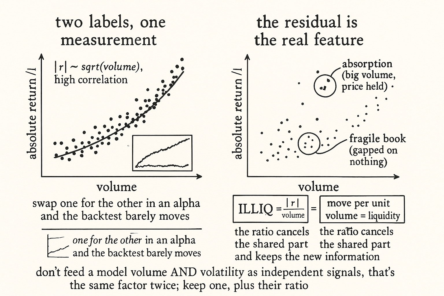
Read it as: the absolute return on a bar scales with the square root of the information arriving that bar, trading volume scales with that same information count, so absolute return scales with the square root of volume. The constant differs by instrument, but the link is mechanical, not coincidental, and it shows up as a high positive correlation between absolute returns and volume in almost every liquid market you measure.

The double-counting trap

Feed volume and volatility into the same model as if they were two separate signals and you have put the same factor in twice. In a linear model this is textbook collinearity: the two columns are nearly the same vector, the regression cannot tell which one earns the coefficient, and it splits the weight between them in an unstable way that flips sign across refits. You think you have two predictors holding the model up. You have one predictor leaning on itself.

The damage is quieter in an ensemble. The old turnover-reduction logic, averaging many variants of the same alpha so the correlated signal survives and the uncorrelated noise cancels, assumes the variants share signal but not noise. Stack a volume-normalized momentum and a volatility-normalized momentum into that average and you have not added breadth. You have doubled the weight on one effect and fooled yourself into thinking the ensemble is more diversified than it is. Check the correlation before you treat two features as independent, or the regularization and the averaging both silently misprice them.

import numpy as np
import pandas as pd

# bars with log returns and volume
r = np.log(df["close"]).diff()
abs_ret = r.abs()
vol = df["volume"]

# the overlap: absolute return vs volume, and vs sqrt(volume)
print("corr(|r|, V)      :", abs_ret.corr(vol))
print("corr(|r|, sqrt V) :", abs_ret.corr(np.sqrt(vol)))

# the orthogonal residual that is NOT shared: Amihud illiquidity
illiq = abs_ret / vol            # move per unit of volume

The first two correlations come back high and positive on liquid data, which is the whole point: the absolute move and the volume are mostly the same column. The interesting line is the last one.

The residual is where the real signal lives

Correlated is not identical, and the gap between them is the feature worth keeping. The part of volume that is orthogonal to volatility, big volume with a small price move, is absorption: someone soaked up a flood of trading without letting price run. The mirror case, a large move on thin volume, is a fragile book that gapped on almost nothing. Neither of those shows up if you carry volume and volatility as redundant twins. Both show up the instant you look at their ratio.

$$ \text{ILLIQ}_t = \frac{|r_t|}{V_t} $$

Read it as: Amihud illiquidity is the absolute return divided by volume, the price move you got per unit of volume traded. Because the numerator and denominator carry the shared information-flow component, dividing one by the other cancels most of it and leaves the residual: how much this market moves for a given amount of trading, which is liquidity itself. That residual is genuinely new information next to plain momentum, where two raw copies of the volatility regime are not. The practical rule that falls out: pick one of volume or volatility as your scale, the way the old ATR-normalization article picked ATR, then add their ratio as a second feature rather than adding the other raw level. One regime column plus one liquidity column beats two regime columns pretending to be different.

Visualizing the overlap

KEY POINTS

• Drop volume in for the volatility denominator in most alpha formulas and the backtest barely changes, because volume and absolute returns are both driven by the same information-arrival clock and move together.
• The mixture-of-distributions link is mechanical: absolute return scales with the square root of volume, so the two carry a high positive correlation in liquid markets.
• Feeding both into one model double-counts the factor: collinearity destabilizes a linear model's coefficients, and stacking volume- and volatility-normalized variants into an ensemble fakes diversification the old signal-averaging logic assumed it had.
• Check the correlation before treating two features as independent, or both regularization and ensemble averaging silently misprice them.
• The residual is the keeper: the part of volume orthogonal to volatility is absorption (big volume, small move) or fragility (big move, thin volume), neither visible if you carry the two as redundant twins.
• Amihud illiquidity, |r| over volume, cancels the shared component and leaves liquidity; pick one scale the way the old ATR-normalization article picked ATR, then add their ratio rather than the other raw level.

References

• The Mixture of Distributions Hypothesis: Volume and Volatility (Clark; Tauchen, Pitts)
• Illiquidity and Stock Returns: Cross-Section and Time-Series Effects (Amihud)
• Trading Volume and Serial Correlation in Stock Returns (Campbell, Grossman, Wang)
• Volume, Volatility, and the Information Content of Trades