3. Robust Systems Lab June 28, 2026 5 min

3.35 Trend and Reversion Are the Same, and OLS Understates Both

Trend and reversion are one process split by the sign of beta. Regress a series on its own lag and OLS understates beta's magnitude in both cases, because the lagged regressor shares error terms with the target. You end up believing in less trend and less reversion than the market carries.

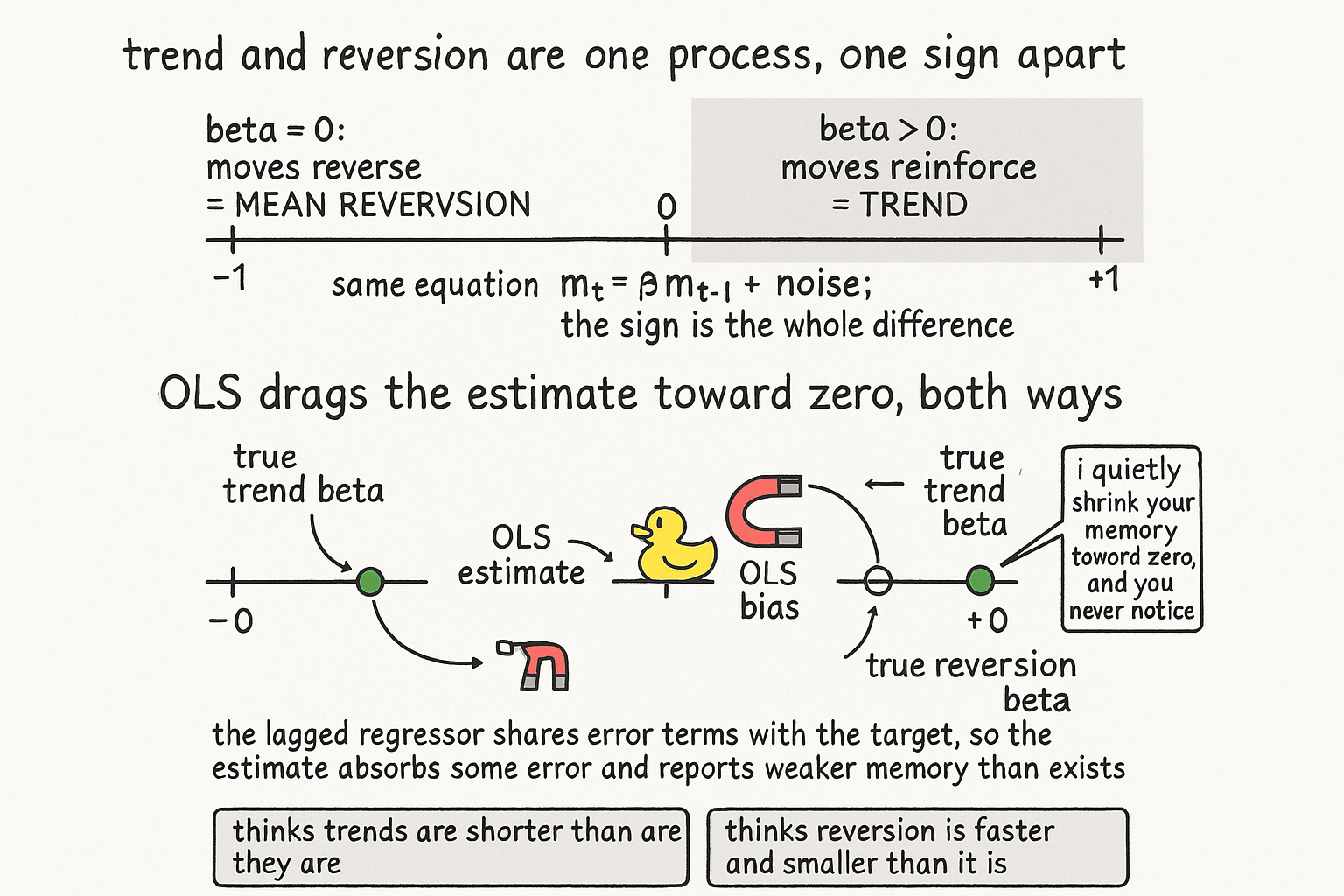
Trend and mean reversion look like opposites, and they are the same process with a sign flipped. Both describe a series whose next value depends on its last value, the only difference being whether the dependence pulls in the same direction or the opposite one. Write the process once and you cover both cases.

$$ m_t = \beta \, m_{t-1} + \varepsilon_t, \qquad \varepsilon_t \sim N(0, \sigma^2) $$

A positive beta means a high value tends to be followed by another high value: moves reinforce, the series trends. A negative beta means a high value tends to be followed by a low one: moves reverse, the series mean-reverts. The variance ratio and the efficiency ratio from the old articles "Variance Ratio Tests for Traders" and "Efficiency Ratio Explained for Traders" are both reading this one number from different angles. One process, one parameter, and the sign of beta is the whole distinction between the two strategy families people treat as separate worlds.

Here is the problem. When you estimate beta from data with ordinary least squares, the estimate is biased toward zero in magnitude, in both the trend case and the reversion case, and the bias is not a quirk of bad data. It is built into the estimator the moment the series has any memory at all.

Where the bias comes from

OLS estimates beta with the same ratio it always uses, the covariance of the series with its own lag over the variance of the lag.

$$ \hat{\beta}_{\text{OLS}} = \frac{\operatorname{Cov}\!\big(m_t,\, m_{t-1}\big)}{\operatorname{Var}\!\big(m_{t-1}\big)} $$

For this ratio to be unbiased, the regressor has to be independent of the error. In a plain cross-sectional regression it is. Here it is not, and the reason is that the regressor is a lagged copy of the thing you are predicting. Expand the series and m_t carries every past shock: epsilon_t, then beta times epsilon_{t-1}, then beta squared times epsilon_{t-2}, and so on back. But m_{t-1} carries the same shocks one step shifted: epsilon_{t-1}, beta times epsilon_{t-2}, and so on. The numerator and the denominator of the OLS ratio share these error terms, because both m_t and m_{t-1} are built out of epsilon_{t-1}, epsilon_{t-2}, and the rest of the history.

That shared dependence is exactly what breaks the unbiasedness condition. In data with no autocorrelation the regressor and error are clean, the ratio is unbiased, and there is no issue. The autocorrelation that makes the series interesting is the same autocorrelation that contaminates the estimator. So the OLS estimate picks up an extra term.

$$ \hat{\beta}_{\text{OLS}} = \beta + \kappa $$

In the trend case, positive beta, the bias kappa is negative, dragging the estimate down. In the strongly reversion case, negative beta, the bias kappa is positive, dragging the estimate up. Both pulls point the same way: toward zero. The estimator absorbs some of the error structure into the coefficient and reports a beta smaller in magnitude than the truth.

What the understatement does to you

The estimate is closer to zero than reality, so the model you build on it believes the series has less memory than it actually has. That single misbelief has two consequences, and they hit trend and reversion alike.

The series converges slower than your model expects. For a trending series, your model expects a shock to decay faster than it truly does, so it underestimates how long a trend persists and exits early. For a reverting series, your model expects the pull back to the mean to happen faster than it truly does, so it underestimates how long the deviation lingers and re-enters too soon. In both cases you have priced in more speed than the process has, because a beta biased toward zero looks like weaker memory, and weaker memory means faster settling.

The model underestimates variance. The magnitude of the next move away from the current level, the size of the swing the process can produce, comes out larger than the biased beta predicts. The old article "Long-Range Dependence: Real Memory or Just Short-Range Echo?" warns about the opposite failure, seeing memory that is not there. This is the mirror: real memory you have measured too small. Underestimating beta's magnitude means underestimating how far the series ranges, so your model predicts weaker reversion than truly happens and shorter trends than truly happen, and it sizes risk against a process calmer than the one you are trading.

Why this matters before you trade either

The practical damage is that both strategy families inherit the same understatement from the same estimator. A trend follower fit with OLS will set its holding period too short and its risk too low. A mean-reversion strategy fit with OLS will set its entry and exit too tight and its variance too low. Neither error announces itself, because the biased beta still fits the in-sample data and still produces a plausible model. The old article "Parameter Stability Beats Best Parameter" makes the broader case that the headline estimate is rarely the number to trust, and this is a clean instance: the point estimate of beta is systematically wrong in a known direction, and you can correct for it.

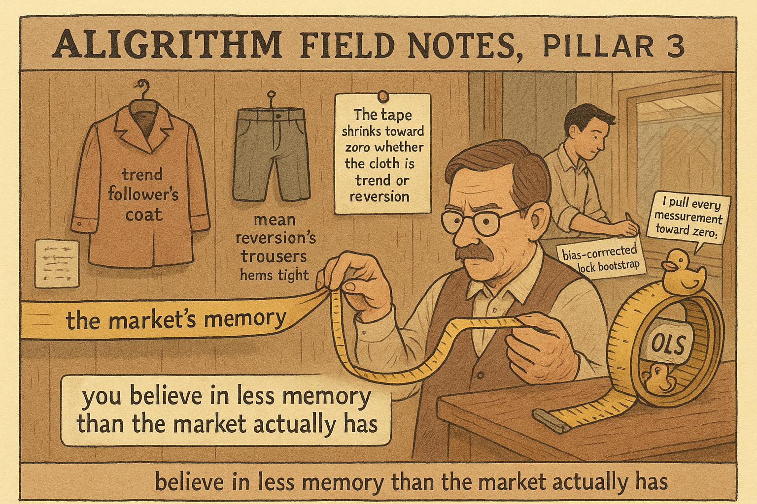
The fixes are standard once you know the bias is there. Small-sample bias corrections for the autoregressive coefficient exist and push the estimate back out toward the truth. Resampling the series in blocks, the same block bootstrap the old article "Variance Ratio Tests for Traders" uses, gives you a distribution for beta that exposes how far the point estimate sits from center. The first move is the recognition: when you regress a series on its own lag, the number that comes back understates the memory, and you are believing in less trend and less reversion than the market actually carries.

Visualizing the understatement

KEY POINTS

Trend and mean reversion are the same first-order process, the next value depending on the last, separated only by the sign of beta. Positive beta reinforces and trends; negative beta reverses and mean-reverts.
OLS estimates beta as the covariance of the series with its lag over the variance of the lag. That ratio is unbiased only when the regressor is independent of the error.
The regressor is a lagged copy of the target, so both share the same past shocks. That shared dependence breaks the unbiasedness condition, and only autocorrelated data has it. The autocorrelation that makes the series tradable is what contaminates the estimate.
The estimate comes out as the true beta plus a bias term. For trends the bias is negative, for strong reversion the bias is positive, and both pull the magnitude toward zero. OLS understates the memory.
A beta too close to zero looks like weaker memory, so the model expects faster settling: trends exit too early, reversion re-enters too soon, and the series actually converges slower than predicted.
The same bias makes the model underestimate variance, predicting weaker reversion and shorter trends than reality and sizing risk against a calmer process. Correct it with small-sample bias adjustments and a block bootstrap, and recognize the understatement before trading either family.

Where the bias comes from

What the understatement does to you

Why this matters before you trade either

Visualizing the understatement

KEY POINTS

References