2. Indicator Engineering June 28, 2026 7 min

2.82 Regularization from First Principles

OLS is the best unbiased fit only under assumptions markets shatter, so on correlated alphas it hands you wild coefficients. Add an L2 or L1 penalty: biased, lower variance, steadier out of sample.

The old article "The Limits of Linear Models" left you with a clean little model that prices the next move off three order-book alphas, something like b_1 times imbalance plus b_2 times order-flow plus b_3 times the microprice tilt. The first question is mechanical: where do b_1, b_2, b_3 come from? You fit them on history. The second question is the one nobody asks until a live model starts drifting: why does the standard way of fitting them, the one every stats course teaches as optimal, fall apart on market data? Regularization is the answer, and you can build it from scratch with nothing fancier than the squared-error objective you already know.

Ordinary least squares, and the theorem that blesses it

Start with the fit itself. You have three noisy alphas x_1, x_2, x_3 and a target, the future price change. You want the coefficients that make the model's predictions match history as closely as possible, so you pick the b_i that minimize the sum of squared errors across all your historical rows.

$$ L \;=\; \sum_{t}\Big(\,b_1 x_{1,t} + b_2 x_{2,t} + b_3 x_{3,t} - y_t\,\Big)^2 $$

Read that as: for every timestamp t, take the model's prediction, subtract the actual future price change y_t, square the miss so big errors dominate and the sign drops out, and add up the squares. The b_i that drive this sum to its minimum are the ordinary-least-squares estimates. This is the workhorse, and there is a theorem that says it is not just convenient but optimal: the Gauss-Markov theorem. It states that among all unbiased estimators that are linear in the data, OLS has the smallest variance. The shorthand is BLUE, the best linear unbiased estimator.

The theorem is real, and the trap is hidden in its fine print. BLUE holds only when three conditions about the model's errors are true: the errors average to zero, they all share one constant variance, and they are uncorrelated with each other. Grant those three and OLS is unbeatable in its class. The whole argument for using it rests on those three assumptions holding.

The assumptions die in markets

Markets violate all three, and not at the margin.

The errors do not share a constant variance. Volatility clusters, so the model's misses are tiny in calm tape and enormous in a vol spike, which is heteroskedasticity by another name, and the old article "Why Volatility Is More Non-Stationary Than Trend" is the long version of why this is the rule rather than the exception. The errors are not even drawn from the same distribution over time, because the relationship you are fitting is non-stationary: the coefficient that priced imbalance well last quarter is wrong this quarter when the book regime shifts. And the tails are fat, so a handful of jump prints carry returns many standard deviations out, which a squared-error objective weights brutally because squaring an outlier makes it scream.

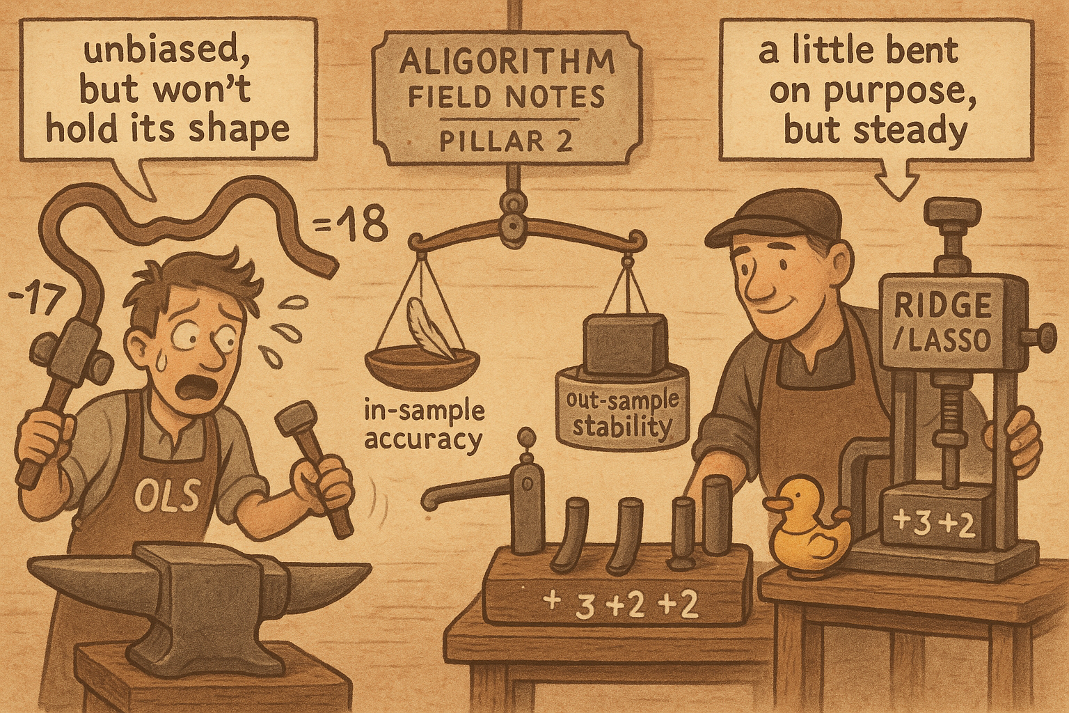
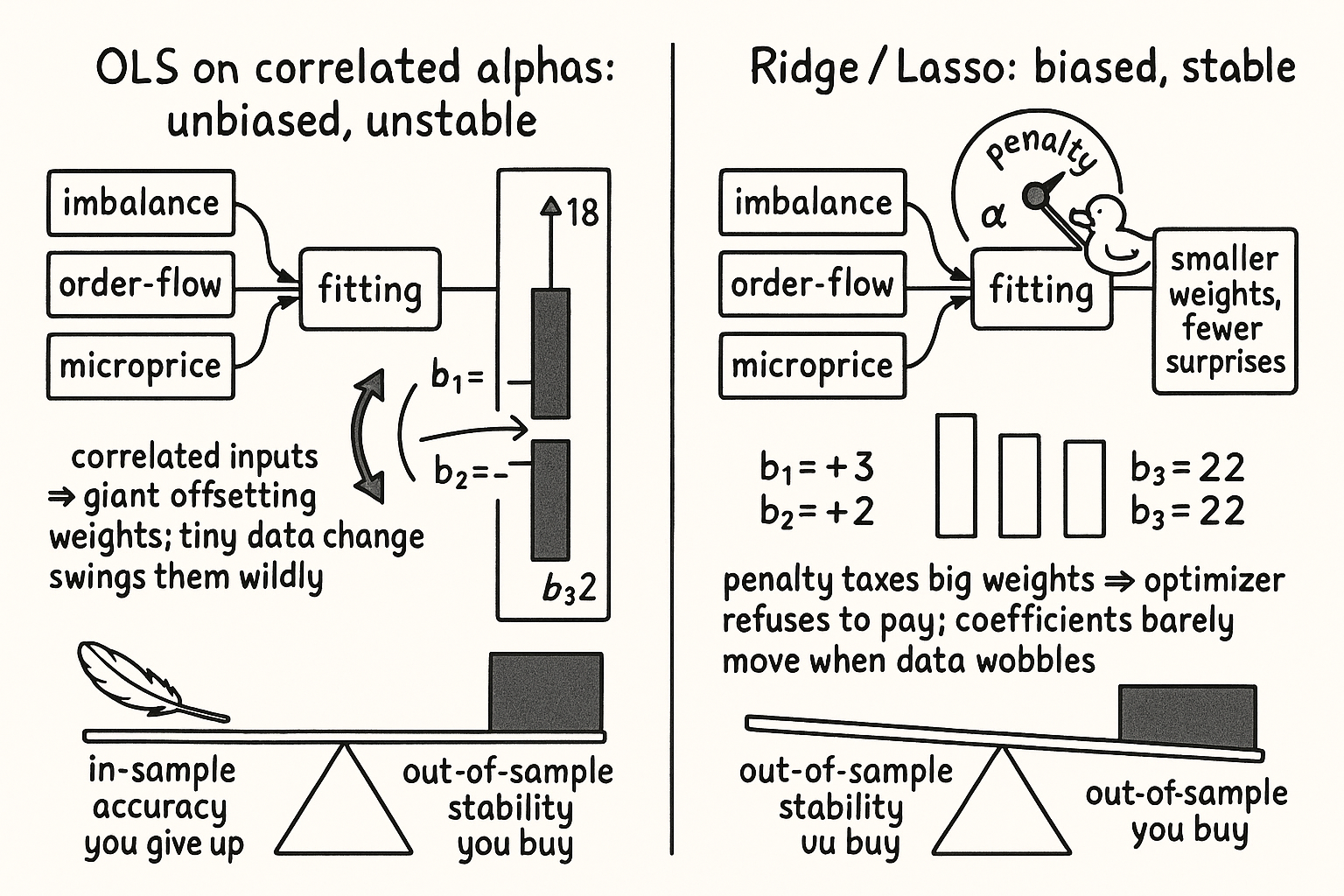
The third violation is the one that matters most for regularization. Your alphas are correlated and redundant. Imbalance, order-flow, and microprice tilt all read the same pressure in the book from slightly different angles, so x_1, x_2, x_3 move together. When the inputs are collinear, OLS cannot tell which one deserves the credit, and it copes by handing out enormous offsetting coefficients, a giant positive b_1 nearly cancelled by a giant negative b_2. The fit looks fine in-sample and the coefficients are garbage: tiny changes in the data swing them wildly, and a coefficient vector that swings on noise prices the next trade on noise.

So the estimates come out unbiased, exactly as the theorem promises, and useless, because their variance is gigantic the moment the inputs are correlated. Unbiased-but-high-variance is the worst trade you can be holding when you have to commit capital to the forecast.

Buy variance back with a penalty

The fix is to stop insisting on unbiasedness. Add a term to the objective that punishes large coefficients, so the optimizer has to weigh fitting the data against keeping the b_i small.

$$ \text{Ridge (L2):}\quad L \;+\; a\,\big(b_1^2 + b_2^2 + b_3^2\big) $$ $$ \text{Lasso (L1):}\quad L \;+\; a\,\big(|b_1| + |b_2| + |b_3|\big) $$

Read the ridge line as: minimize the same sum of squared errors as before, but add a tax equal to a constant a times the sum of the squared coefficients. The lasso line taxes the sum of the absolute coefficients instead. In both, a is a dial you set: at a equal to zero you are back to plain OLS, and as a grows the penalty drags every coefficient toward zero. Those offsetting giant coefficients that collinearity produced are now expensive, so the optimizer refuses to pay for them and settles on a smaller, steadier set.

This estimator is biased. The Gauss-Markov theorem no longer applies and you would not have been allowed to use this before, because shrinking the coefficients pulls the fit away from the in-sample optimum on purpose. The trade is bias for variance: you give up a sliver of in-sample accuracy and buy back a large chunk of stability, so the coefficients barely move when the data wobbles and the out-of-sample forecast holds up. The old article "Parameter Stability Beats Best Parameter" is the same discipline applied to a different knob, and it is the discipline that the whole machine-learning arc keeps coming back to.

Ridge spreads, lasso selects

The two penalties shrink differently, and the difference decides which to reach for.

Ridge squares the coefficients, so the marginal tax on a coefficient grows as it grows, which makes ridge punish a few large weights far more than many small ones. Faced with three correlated alphas, ridge spreads the weight across all three rather than letting one blow up, which is what you want when you believe every input carries a little real signal and you want a smooth, stable blend.

Lasso taxes the absolute value, and the geometry of that penalty drives weak coefficients exactly to zero rather than merely small. Lasso does feature selection: hand it ten redundant momentum variants and it tends to keep one and zero the rest. That is useful when you suspect most of your inputs are noise and you want a sparse model, and it is dangerous with correlated alphas because which one survives can flip from one sample to the next, so the selection itself becomes a source of instability.

A common practical answer is to mix the two, an L1 plus L2 blend, which gets lasso's sparsity without its arbitrary tie-breaking among correlated inputs. The choice is not cosmetic: it encodes what you believe about your alphas, whether they are many weak real signals to be blended or a noisy pile to be pruned.

Setting the dial without cheating

The penalty strength a is a parameter, which means it is one more thing you can overfit if you pick it by staring at the in-sample fit. At a equal to zero the in-sample error is always lowest, because that is what OLS minimized, so the in-sample curve will always tell you to regularize less, which is exactly backwards. You set a out of sample. Cross-validate across folds, or walk it forward, and watch the held-out error as you raise a: it falls as shrinkage kills the variance, bottoms out, and climbs again once you have shrunk so hard the model can no longer fit the real structure. You want the floor of that held-out curve, not the floor of the in-sample one, and you want to read it as a plateau rather than a spike, the same way the old article "The Hill, the Spike, and the Cliff: Reading Optimization Surfaces" tells you to read any optimization surface.

Where this sits in the arc

Regularization is the linear model's variance medicine, and it is the same medicine the next articles give to trees. The old article "From One Tree to Forests to Boosting" stabilizes a fragile tree by averaging many of them, which is a variance cut by a different mechanism, and boosting's learning rate is a shrinkage knob in disguise, a per-step tax that keeps each tree from overcommitting. Ridge and lasso are where the idea is cleanest, because you can see the penalty sitting right next to the squared-error term and watch it trade bias for stability one coefficient at a time. Carry that picture forward: every model past the toy linear one is going to need some version of this brake, and the reason is always the same, that an unbiased fit on non-stationary, fat-tailed, collinear market data hands you a high-variance answer you cannot trade.

Visualizing the trade

KEY POINTS

Fitting a linear alpha model means minimizing squared error, and the Gauss-Markov theorem says that fit, OLS, is the best linear unbiased estimator. The blessing holds only under three assumptions: zero-mean errors, constant variance, and uncorrelated errors.
Markets break all three. Volatility clustering kills constant variance, regime shift kills stationarity, fat tails make squared error chase outliers, and correlated alphas make OLS hand out giant offsetting coefficients that swing on noise.
Unbiased but high-variance is a bad hand to hold when you have to trade the forecast. The fix is to drop unbiasedness on purpose.
Add a penalty: ridge taxes the sum of squared coefficients, lasso taxes the sum of absolute coefficients, with a dial a setting the strength. The estimator becomes biased but far lower variance and steadier out of sample.
Ridge spreads weight across correlated inputs for a smooth blend; lasso drives weak weights to zero for a sparse model but picks arbitrarily among correlated inputs. An L1+L2 blend gets sparsity without the arbitrary tie-break.
Set a out of sample, never in sample, where the error always favors a equal to zero. Cross-validate or walk forward and take the plateau of the held-out error.
This is the linear-model version of the variance cut that bagging and boosting give to trees. Every model past the toy linear one needs some version of this brake.