5.46 Bid-Ask Spread From OHLC: The GMM Estimator That Beats Roll/CS
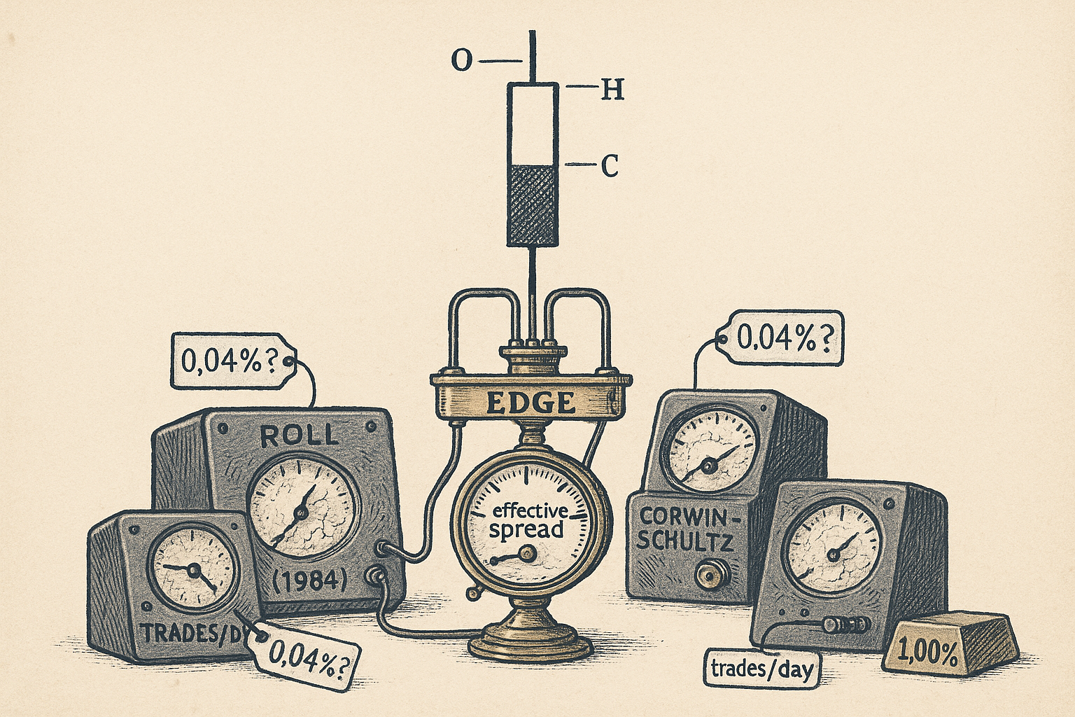
Your backtest's "spread" is probably a continuous-time estimate that reads 0.04% on a real 1.00% cost when trading is thin. EDGE fixes the discreteness bias from OHLC alone and beats Roll and CS.
You backtest a strategy, subtract "a spread" for costs, and move on. Where did that number come from? If you typed in a guess, or pulled a single quoted spread from a vendor, you are almost certainly wrong, and wrong in the one direction that flatters your worst assets. The effective spread you actually pay is unobservable without trade-and-quote data, and quote data for anything outside recent U.S. large-caps is expensive, patchy, or nonexistent. So most people estimate the spread from the only thing they have: open, high, low, close candles. The problem is that the popular estimators for doing that were built on an assumption that is false in exactly the markets where costs bite hardest.
The old article "Why Transaction Costs Should Be Added Before You Fall in Love" argued you must apply realistic costs from the prototype stage, before you get emotionally attached to a pre-cost Sharpe. This article is the missing piece of that: how to get the spread number honestly from OHLC alone. David Ardia, Emanuele Guidotti, and Tim Kroencke derive an estimator they call EDGE, the Efficient Discrete Generalized Estimator, and show it dominates the seminal Roll estimator and the more recent Corwin-Schultz and Abdi-Ranaldo estimators across simulations and 1.6 million stock-months of real data. The single number that should make you nervous: when trading is thin, Corwin-Schultz reports a spread of 0.04% where the true spread is 1.00%. That is not a small error. That is your cost model understating reality by a factor of 25 on precisely the illiquid names where the spread is the whole game.
What "effective spread" even means
Start with the thing being estimated, because half the confusion in cost modeling is people measuring different quantities and calling them the same word. The relative effective spread for a single trade is the distance between the price you got and the true, unobserved fundamental value.
$$ S = \frac{2D(P - \bar{P})}{\bar{P}} $$
S is the relative effective spread, P is the transaction price you actually paid, P-bar is the unobserved fundamental price, and D is a direction indicator that is plus one for a buyer-initiated trade and minus one for a seller-initiated trade. The factor of two turns a one-sided distance from the midpoint into a full round-trip spread. Work a number: you buy at 100.10, D is plus one, and the fundamental price is 100.00. Then S is 2 times 1 times (100.10 minus 100.00) divided by 100.00, which is 0.20 divided by 100, or 0.20%. If you had instead sold at 99.90 with D minus one, you would get the same 0.20%. The catch is right there in the formula: P-bar is unobservable. Every estimator in this fight is just a different way of guessing it. High-frequency methods proxy P-bar with the quoted midpoint from actual quote data. Low-frequency methods, the subject here, assume a model of how prices move and back the spread out of transaction prices alone.
The old guard, and why they break
The low-frequency lineage starts with Roll in 1984. His insight: if the fundamental price is a random walk and trades bounce between bid and ask, then consecutive observed price changes are negatively correlated, and the size of that negative serial covariance tells you the spread.
$$ S^2 = -4\,\mathrm{Cov}[\Delta c_t, \Delta c_{t-1}] $$
The squared spread equals minus four times the serial covariance of consecutive close-to-close log-return changes, where delta-c-t is the change in the closing log-price from one period to the next. Plain version: the bid-ask bounce makes an up-tick tend to follow a down-tick, that alternation shows up as negative covariance, and Roll inverts it to recover the spread. Worked example: if the covariance of consecutive daily close changes is minus 0.000025, then S-squared is minus four times minus 0.000025, which is 0.0001, and S is the square root, 0.01, or 1.00%. The fatal weakness is variance. On a yearly sample of daily closes that covariance is so noisy it comes out positive about half the time, which makes S-squared negative, which is nonsense, so you truncate to zero and throw away half your estimates. Corwin-Schultz improved on Roll using the high-low range, and Abdi-Ranaldo improved again using close plus the high-low midpoint, each with lower variance. But all three share one buried assumption: that prices are observed continuously, meaning there is always at least one trade between any two observations. That assumption is the crack the whole edifice falls through.
The discreteness fix nobody else made
Real markets are discrete. Some days a thin stock trades a handful of times; some intraday bars have zero trades and the OHLC just gets forward-filled from the previous close. When that happens, the observed price stops bouncing, the negative serial covariance shrinks, and every continuous-time estimator reads that as a smaller spread. It is not smaller. It is undersampled. The authors' contribution is an analytical correction: the probability that the open or close price coincides with the high or low. Under continuous observation that probability is zero. In reality it ran between 25% for large stocks and 75% for small stocks over 1926 to 2021, and it climbs as you move to intraday sampling where each bar holds fewer trades. The corrected spread-at-open estimator looks like this.
$$ S_o^2 = \frac{-8\,\mathbb{E}[(\eta_t - o_t)(o_t - c_{t-1})]}{\mathbb{P}[o_t \neq h_t] + \mathbb{P}[o_t \neq l_t]} $$
The squared spread at the open equals minus eight times the expected product of two returns, the mid-to-open return and the open-to-previous-close return, divided by a correction term: the probability that the open differs from the high plus the probability that the open differs from the low. Here o, h, l, c are open, high, low, close log-prices and eta is the high-low midpoint. The numerator is the same covariance idea as Roll and Abdi-Ranaldo. The denominator is the fix. When trading is frequent, open rarely equals high or low, both probabilities are near one, the denominator is near two, and you recover the classic estimator. When trading is thin, open often equals the high or the low, the probabilities shrink, the denominator shrinks, and dividing by a smaller number scales the estimate back up to where it belongs. Worked example: suppose the raw covariance term gives a numerator implying an uncorrected S-squared of 0.36 (a 0.60% spread), but the stock is thin so the probability the open differs from the high is 0.6 and from the low is 0.6, summing to 1.2 instead of 2.0. The corrected estimate is scaled by 2.0 over 1.2, lifting S-squared to 0.60 and the spread to about 0.77%. The continuous-time estimator would have reported the 0.60% and quietly understated your cost.
Combine everything, optimally
One estimator uses open, high, low. You can build others from different price combinations: close-high-low, open-high-low-close, close-high-low-open. The authors derive four such building blocks and prove something useful about them. Two of them (the open-high-low-close and close-high-low-open versions) have the lowest variance when the spread is small relative to volatility. The other two (open-high-low and close-high-low) win when the spread is large relative to volatility. No single one is best everywhere. So rather than pick, they combine all four using the generalized method of moments from Hansen 1982: write each estimator as a moment condition and blend them to minimize the variance of the result. The efficient combination weights each piece inversely to its variance.
$$ S_{EDGE}^2 = w_1\,\mu_1 + w_2\,\mu_2, \qquad w_i \propto \frac{1}{\mathrm{Var}[x_i]} $$
The EDGE estimate is a weighted average of the moment estimates mu-1 and mu-2, where each weight is proportional to the inverse of that estimator's variance, so the more precise building block gets more say. Plain version: it is the same logic as combining two noisy measurements of the same thing by trusting the tighter one more. Worked example: say estimator one has variance 4 and estimator two has variance 1. The raw inverse-variance weights are 0.25 and 1.0, which normalize to 0.20 and 0.80. If estimator one reads 0.90% and estimator two reads 0.95%, EDGE reports 0.20 times 0.90 plus 0.80 times 0.95, which is 0.94%, leaning hard on the precise estimator. Because the low-variance building blocks are different for small and large spreads, EDGE automatically shifts its weight toward whichever pair is trustworthy in the current regime, which is how it achieves minimum variance across both. That regime-adaptive weighting is the "efficient" in Efficient Discrete Generalized Estimator, and it is what lets a single formula beat Roll and CS everywhere instead of just somewhere.
Does it work: the simulation
The authors run the standard Corwin-Schultz simulation setup: 10,000 months, 21 trading days each, 390 minutes a day, a fundamental price on a geometric random walk with 3% daily volatility, and a bid-ask bounce of a known size. Then they vary how often a trade is actually observed, from every minute down to roughly once a day, and check whether each estimator recovers the true 1.00% spread.
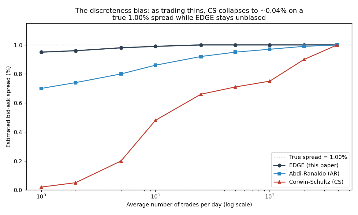
At 390 trades a day, everyone is fine: all estimators land near 1.00%. As trading thins, the story splits hard. Corwin-Schultz reads 0.75% at 100 trades a day and craters toward zero below ten trades a day, bottoming near 0.04% in the sparse simulations. Abdi-Ranaldo is less sensitive but still sags below the truth. EDGE stays flat at 1.00% down to roughly a single trade per day. The variance results are just as decisive: across simulated spreads from 0.50% to 8.00%, EDGE has the lowest standard deviation of any estimator, uniformly, small spreads and large. It wins on bias when others are biased, and it wins on precision when everyone is unbiased.
Does it work: the real data
Simulations can be rigged to flatter the home team, so the empirical test matters more. The authors take every U.S. common stock in CRSP from 1993 to 2021, about 1.64 million stock-months, estimate the spread from daily OHLC with each method, and compare against a ground-truth effective spread built by matching high-frequency trades to quotes in the TAQ database, the Holden-Jacobsen benchmark.
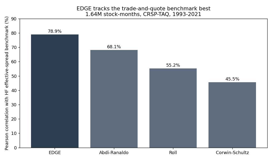
EDGE hits 78.9% Pearson correlation with the benchmark. Abdi-Ranaldo manages 68.1%, Roll 55.2%, and Corwin-Schultz only 45.5%. EDGE also posts the lowest mean absolute percentage error, 16.2% against CS's 35.9%, and the smallest fraction of non-positive estimates. It wins in every subsample the authors slice: every market venue, every sub-period, every size decile, every spread-size bucket, and every trading-frequency group. One more finding worth carrying into your cost model: the end-of-day quoted spread runs about double the effective spread, because dealers routinely trade inside their own quotes. If you have been costing trades at the quoted spread, you have been roughly doubling your assumed transaction cost, which is conservative but wasteful for sizing.
The frequency upgrade that reconciles two literatures
Here is the part that should interest anyone doing microstructure work. Because EDGE handles discreteness correctly, you can feed it intraday candles instead of daily ones and it just gets better, where the old estimators break. On the hard sample from October 2003 to December 2021, where spreads are tiny relative to volatility and daily estimates are noisy, switching EDGE from daily to minute OHLC does this.
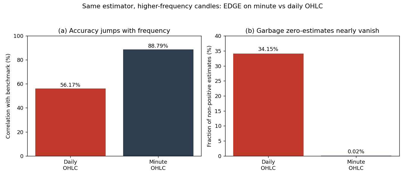
Correlation with the benchmark jumps from 56.17% to 88.79%. The fraction of non-positive estimates, the garbage zeros you have to truncate, falls from 34.15% to 0.02%, so the upward bias that truncation induces essentially disappears. And it is more effective to raise the sampling frequency than to pile on more years of daily data. That is the reconciliation: the same estimator spans the low-frequency and high-frequency literatures depending on what candles you feed it. Outside equities it holds too. For cryptocurrencies, the old estimators produce a tenfold gap between daily and intraday estimates, a clear sign of the discreteness bias, while EDGE's daily estimates overlap its hourly and minute estimates. For a 24/7 asset with no official quote feed, an estimator that gives the same answer at any frequency is close to the only honest option.
How to use it, and where it stops
Practically, this is not a research toy you have to reimplement. The authors ship it as the open-source bidask package in R, Python, C++, and more. You hand it a frame of open, high, low, close columns and it returns the effective spread for the window. Then it drops straight into the net-edge accounting from the old article "Why Transaction Costs Should Be Added Before You Fall in Love": net edge is gross edge minus cost, and EDGE gives you a defensible, asset-specific, frequency-appropriate estimate of the largest slice of that cost without paying for quote data.
Now the honest limits, because a spread estimator is not a cost model. First, EDGE estimates the average effective spread over the estimation window, not the spread on your specific fill at your specific size. It is a population parameter, not a quote. Second, it rests on the standard assumptions that fundamental returns are serially uncorrelated and that bid-ask bounces are zero-mean and uncorrelated with those returns; strong intraday autocorrelation, momentum, or jumps violate those and will bias it, so it is a spread estimator, not a free lunch. Third, negative estimates still get truncated to zero, so in very small samples a residual upward bias survives even for EDGE, which is why more data or higher frequency helps. Fourth and most important, the effective spread is only one cost term. It does not capture market impact, the extra price you move by trading size, which is a separate and often larger cost for anyone trading meaningful volume. That is the domain of the old article "Market Impact and the Square-Root Law: Walking the Book to Price Your Slippage." Your real per-trade cost is commission plus effective spread plus impact. EDGE nails the middle term cheaply and honestly; you still owe the other two.
Where this connects
For Pillar 5, this is the cheapest reliable microstructure measurement you can make: liquidity, quantified from the candles you already have, at whatever frequency you sample, across asset classes that never had quote data. For the data and backtesting work, it is a direct upgrade to your cost assumptions, and it kills a real source of what the literature calls non-standard errors, the silent variation in results caused by everyone estimating costs differently. The uncomfortable lesson underneath all of it: the "spread" in your backtest was probably a continuous-time estimate that understated the cost of your thinnest, most seductive-looking assets, and understating cost on illiquid names is exactly how a strategy looks profitable on paper and bleeds in production.
KEY POINTS
- The effective spread is the distance of your fill from the unobserved fundamental price, S equals 2D times (P minus P-bar) over P-bar. Every low-frequency estimator is just a different guess at the fundamental price from OHLC data.
- Roll, Corwin-Schultz, and Abdi-Ranaldo all assume prices are observed continuously. Real markets are discrete, and when trading is thin those estimators are downward biased, understating the spread exactly when it is largest.
- EDGE's fix is an analytical correction term: the probability that the open or close equals the high or low. That probability is zero under continuous observation but ran 25% to 75% for real stocks, and it rescales the estimate back to unbiased.
- EDGE combines four OHLC building blocks via GMM (Hansen 1982), weighting each inversely to its variance, so it achieves minimum variance across both small and large spreads instead of winning only in one regime.
- In simulation, Corwin-Schultz reads 0.04% on a true 1.00% spread when trading is thin; EDGE stays unbiased down to about one trade per day and has the lowest variance uniformly.
- On 1.64 million CRSP-TAQ stock-months, EDGE hits 78.9% correlation with the trade-and-quote benchmark versus 68.1% (AR), 55.2% (Roll), and 45.5% (CS), and wins in every venue, period, size, and frequency bucket.
- Feeding EDGE minute instead of daily candles lifts correlation from 56.17% to 88.79% and cuts non-positive estimates from 34.15% to 0.02%, reconciling low- and high-frequency spread measurement in one estimator, and it holds up on crypto where the others show a tenfold daily-vs-intraday gap.
- It measures the average effective spread, not your fill and not market impact. Use it for the spread term of your cost model, then add commission and impact separately.
References
- The Art of Currency Trading - Brent Donnelly (Amazon)
- Efficient estimation of bid–ask spreads from open, high, low, and close prices (Efficient estimation of bid–ask spreads from ohlc)
A note on AI. The ideas, research, analysis, and conclusions in this article are my own. I use AI tools to help with editing and wordsmithing, because English is not my first language, and I am not shy about that. AI-generated ideas and AI-assisted writing are not the same thing: the first is empty slop from a generic prompt, the second is a tool for communicating years of real research more clearly. Judge the work by its substance, not by whether software helped polish the prose.