2.71 Normalized On-Balance Volume
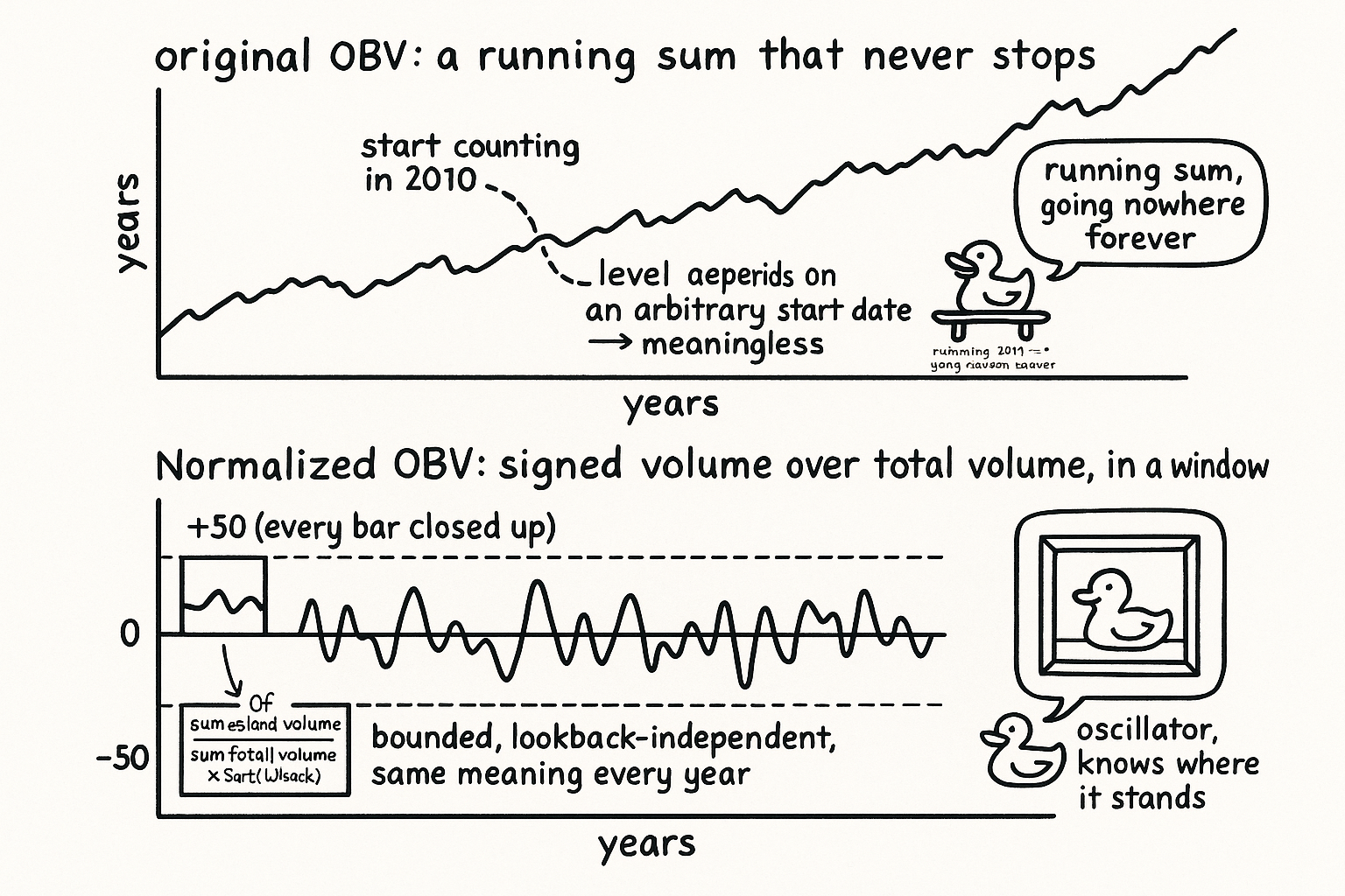
OBV's running sum wanders like a random walk and depends on when you started counting. Window it, divide signed volume by total volume, scale by root-lookback, and you get a bounded, stationary flow oscillator.
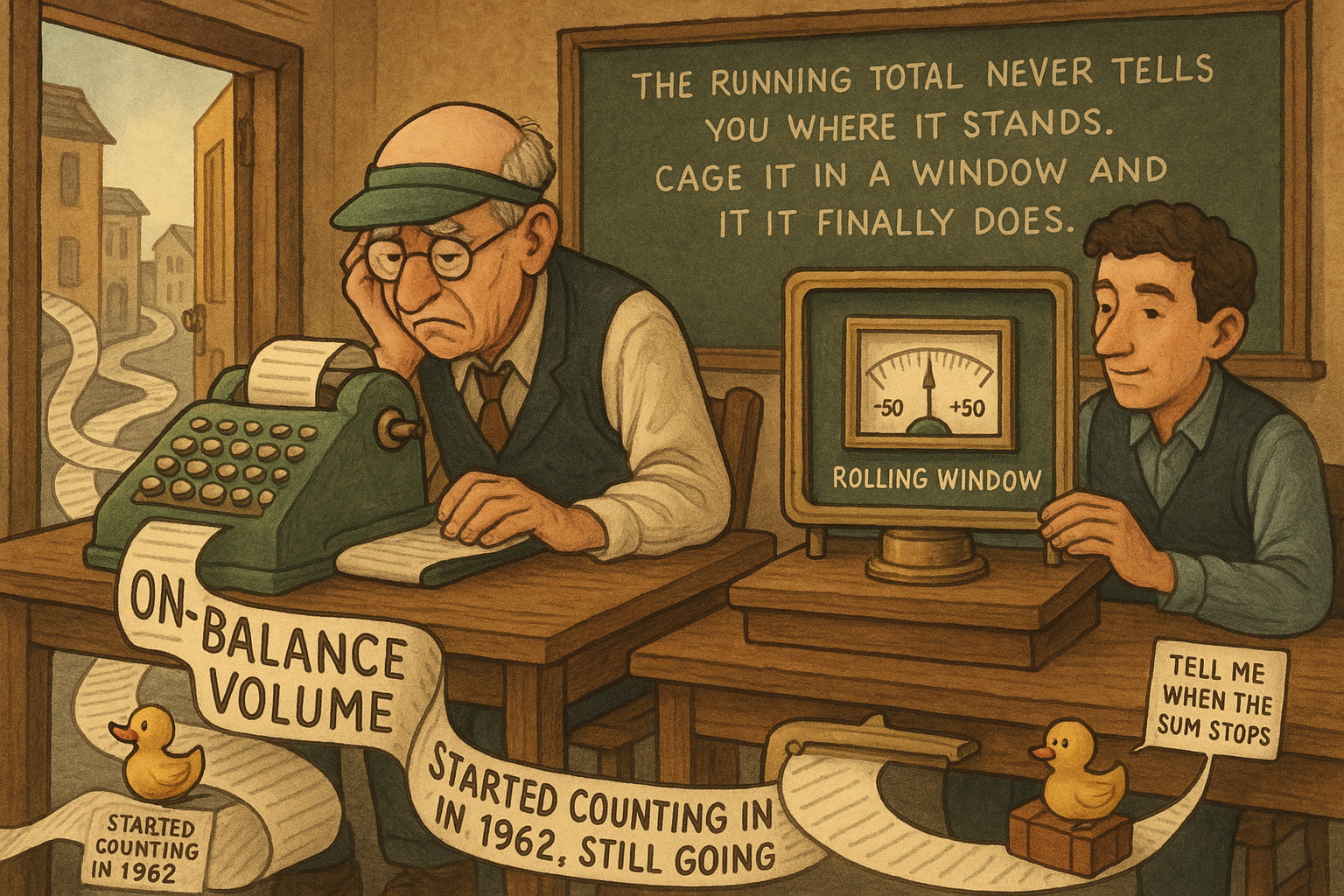
On-Balance Volume has survived since the early 1960s on a single idea that sounds reasonable: when price rises, add the day's volume to a running total, and when it falls, subtract it. The running total is supposed to reveal whether volume is quietly accumulating behind up moves or down moves before price confirms it. Joseph Granville built a following on this, and the indicator still ships in every charting package. As a number you feed a model, it is broken. The running sum wanders like a random walk, its level depends on how many years ago you started counting, and its variance balloons as market volume grows. This article keeps Granville's signed-volume insight and throws away the running sum, rebuilding OBV into a bounded oscillator that means the same thing on any instrument in any decade.
The original, and why the running sum poisons it
The construction is one line. Look at the sign of the close-to-close change, then add or subtract the full bar volume from a cumulative total.
$$ \text{OBV}_t = \text{OBV}_{t-1} + \operatorname{sign}(C_t - C_{t-1}) \cdot V_t $$
The signed-volume idea is sound. Volume on up bars and volume on down bars are different evidence, and tracking which side the volume lands on is a real question. The cumulative wrapper destroys it. A running sum of signed volume has no fixed level, so its current value depends entirely on the arbitrary date you began accumulating; start in 2010 and start in 2015 and you get two completely different OBV levels on the same bar today. Worse, because volume grows over the years, both the local mean and the local variance of the sum drift upward without bound, and the path itself wanders like a near-random walk with no tendency to return to any reference. The old article "The Case Against Raw Price Indicators" condemned raw price for being non-stationary in mean and variance and incomparable across instruments; cumulative OBV fails all three the same way, and a momentary OBV reading carries no usable information because there is nothing to compare it against.
Cage it in a window, then divide out the volume
Two changes fix it. First, stop accumulating forever and compute the signed volume only over a rolling lookback window. A windowed sum cannot wander off to infinity; old bars fall out the back as new ones enter, so the quantity behaves like an oscillator instead of a random walk. Second, kill the variance non-stationarity by dividing the signed volume in the window by the total volume in the same window. The growing volume scale sits in both numerator and denominator, so it cancels, and the result is a ratio that lives on a fixed axis.
$$ \text{Ratio} = \frac{\sum_{k=0}^{LB-1} \operatorname{sign}(C_k - C_{k+1}) \cdot V_k}{\sum_{k=0}^{LB-1} V_k} $$
Read the bounds and the meaning falls out. If every bar in the window closed up, every term in the numerator carries a positive sign and the numerator equals the denominator, so the ratio pins at plus one. If every bar closed down the ratio pins at minus one. Anything in between measures how cleanly volume aligns with direction: near plus one means the up bars carried the volume, near minus one the down bars did, near zero means volume split evenly across up and down bars with no net flow. This is the same cancellation that built Chaikin Money Flow in the old article "Intraday Intensity and Chaikin Money Flow, Made Stationary", applied to signed volume instead of close-position-weighted volume. The old article "How to Build Stationary Indicators from Non-Stationary Prices" is the general principle: divide two quantities that grow together and the growth disappears.
Make it independent of the lookback, then tame the tails
The bounded ratio is already a decent indicator, and it has one more flaw worth removing. Its variance depends on the window length. A short lookback samples few bars, so the ratio swings hard toward the extremes; a long lookback averages more bars, so it hugs zero. That means a reading of 0.4 from a 10-bar window and a reading of 0.4 from a 100-bar window are not the same event, which breaks comparability across settings. The variance of the ratio runs inversely with the number of bars, so multiplying by the square root of the lookback rescales every window to a common spread. The old article "Why ATR Normalization Is More Than a Volatility Trick" used the same square-root-of-lookback divisor to cancel horizon dependence in price momentum; here it cancels horizon dependence in volume flow.
After the square-root rescaling, pass the result through a normal-CDF compression to pull rare outliers into a bounded range and rescale to a clean plus or minus fifty.
$$ \text{NormOBV} = 100 \cdot \Phi\!\left(\sigma_0 \sqrt{LB} \cdot \text{Ratio}\right) - 50 $$
The term inside is the lookback-normalized ratio, scaled by a constant so the bulk of the distribution lands in the linear region of the CDF rather than saturating against its knees. Phi is the standard normal CDF, the same bounded squashing transform the old article "Taming Indicator Tails with Sigmoid Transforms" recommended, chosen here because it maps the whole real line into a fixed interval while leaving the body of the distribution roughly linear. The minus fifty recenters the output so it swings symmetrically around zero. The result is a volume-flow oscillator on a fixed minus-fifty to plus-fifty axis whose meaning does not shift with the lookback, the instrument, or the year.
The change matters more than the level
One operational note that applies more to the original than the rebuild. With cumulative OBV, traders watched the slope, the bar-to-bar change, far more than the absolute level, because the level was meaningless and only the direction of accumulation carried any signal. That habit was a workaround for a broken indicator. With the normalized version the level itself is meaningful, since it is a bounded, stationary reading of how volume aligns with direction over the window, so you can use the value directly. The delta still carries information, a sharp move in the normalized OBV flags a regime shift in who is carrying the volume, but you are no longer forced to read the change because the level finally means something on its own.
KEY POINTS
- Original OBV adds the bar's volume to a running total on up closes and subtracts it on down closes; the signed-volume idea is sound but the cumulative wrapper makes the level depend on an arbitrary start date and wander like a random walk.
- Cumulative OBV is non-stationary in mean and variance and incomparable across instruments, the exact failures the old article "The Case Against Raw Price Indicators" warned about, so a momentary reading carries no usable information.
- Replacing the endless sum with a rolling-window sum stops the wandering and turns the indicator into an oscillator; dividing the windowed signed volume by the windowed total volume cancels the growing volume scale, the trick from the old article "How to Build Stationary Indicators from Non-Stationary Prices".
- The resulting ratio is bounded in minus one to plus one: plus one when every bar in the window closed up, minus one when every bar closed down, zero when volume splits evenly across direction.
- The ratio's variance runs inversely with the lookback, so multiplying by the square root of the lookback makes it independent of the window, the same horizon-cancelling move as the old article "Why ATR Normalization Is More Than a Volatility Trick".
- A normal-CDF compression tames outliers and rescales to plus or minus fifty, following the old article "Taming Indicator Tails with Sigmoid Transforms"; the normalized level is meaningful on its own, so you no longer have to read only the slope.