4. Market Structure Notes June 27, 2026 8 min

4.66 Granger Causality: Finding What's Driving Your Currency Right Now

Your currency's driver rotates by regime, so a fixed watchlist goes stale. Granger causality asks which candidate actually improves the forecast right now, run multivariate so the dollar doesn't fool you.

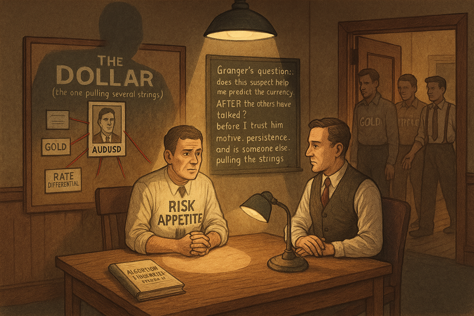
A trader is long AUDUSD and wants to know what to watch on the second screen. The textbook answer is a fixed list: gold, copper, iron ore, the S&P 500, the Australia-US rate differential. The old article "Why FX Traders Must Watch Gold, Rates, and Equities" built that list and turned it into a confirmation count. The list is correct and useless at the same time, because it names every driver that has ever mattered for the Aussie and stays silent on the one that matters this week. Risk appetite drives it in a panic, the rate differential drives it in a calm tightening cycle, copper drives it when China is the story. The driver rotates, and a static list does not tell you where you are in the rotation.

Granger causality is the tool that picks the live driver out of the candidate set. It does not prove that copper causes AUDUSD in any physical sense. It asks a narrower, testable question: does knowing copper's recent moves help me predict AUDUSD better than AUDUSD's own past alone? If the answer is yes, copper "Granger-causes" AUDUSD over that window, and that is exactly the relationship a confirmer or a lead-lag tilt wants to exploit. The old article "Lead-Lag Relationships in Global Markets" measured a single lead with a lagged cross-correlation; Granger generalizes it to a regression that handles several lags at once and, crucially, lets you condition on the other candidates so you do not get fooled by a hidden third variable.

The bivariate test: does X improve the forecast of Y?

Start with two series, candidate driver x (say copper returns) and your currency y (AUDUSD returns). Fit two forecasting models of y. The first uses only y's own past, the restricted model. The second adds lagged values of x, the unrestricted model.

$$ \text{Restricted:}\quad y_t = a_0 + \sum_{i=1}^{p} a_i\, y_{t-i} + e_t $$ $$ \text{Unrestricted:}\quad y_t = a_0 + \sum_{i=1}^{p} a_i\, y_{t-i} + \sum_{j=1}^{p} b_j\, x_{t-j} + u_t $$

Both models predict today's return on the currency from the last p bars. The restricted model is allowed to use only the currency's own history. The unrestricted model also gets the last p bars of the candidate driver, with the coefficients b_j measuring how much each lag of x pulls on y. The whole test reduces to one question about those b coefficients: are they jointly different from zero, or is the candidate adding nothing the currency's own past did not already contain?

Measure it by how much the added series shrinks the prediction error. Collect the sum of squared residuals from each model and compare.

$$ F = \frac{(\text{RSS}_R - \text{RSS}_U)/p}{\text{RSS}_U/(N - 2p - 1)} $$

RSS_R is the squared error of the restricted model and RSS_U the squared error of the unrestricted one. Adding x can only lower the error or leave it flat, so RSS_R is always at least RSS_U; the numerator is the chunk of error the candidate driver killed, spread over the p lags it cost you. The denominator is the error that remains, per remaining degree of freedom, with N the number of bars. A worked feel for the number: say the currency's own past leaves RSS_R = 1.000 over a window, and adding copper drops it to RSS_U = 0.940 with p = 3 lags and N = 250 bars. The numerator is (1.000 - 0.940)/3 = 0.020, the denominator is 0.940/243 = 0.00387, so F is about 5.2. Against an F distribution with 3 and 243 degrees of freedom that clears the 1% threshold, so copper Granger-causes AUDUSD over that window. The driver is live.

Flip x and y and run it again. Granger causality is directional, and you want the direction where the external market leads the currency, not the one where the currency leads the external market. Often both directions test positive, which is its own warning, covered below.

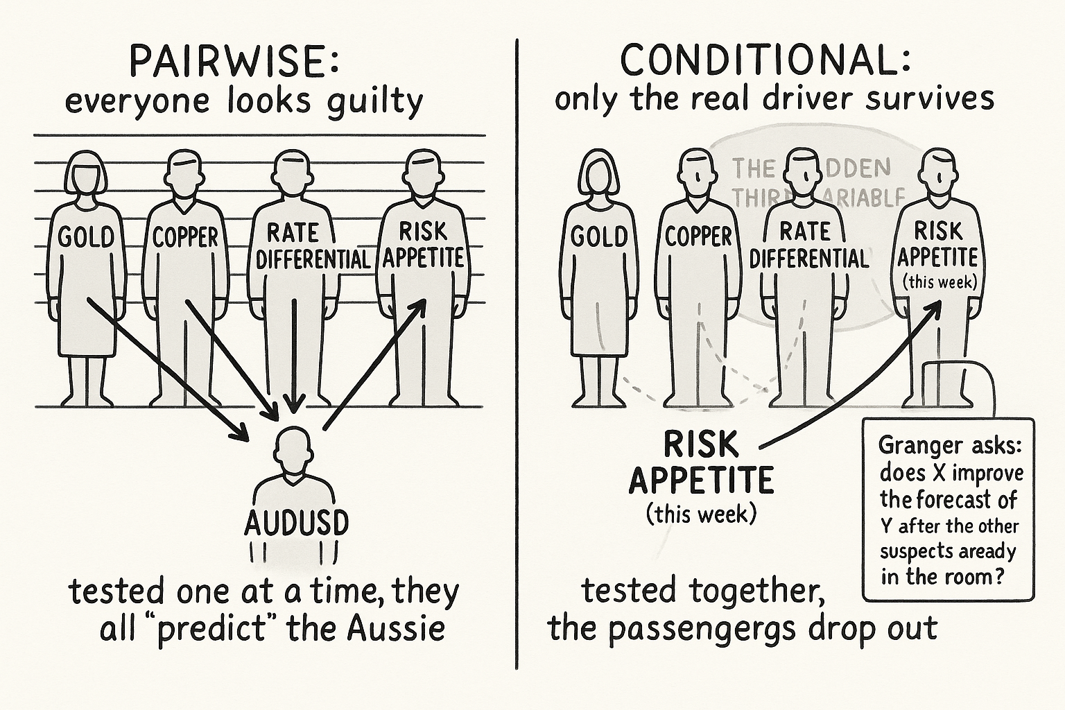
Multivariate: condition on the other suspects to kill the third-variable trap

The bivariate test has the same hole as every correlation in this pillar. Two series can both be driven by a third, and the pairwise test will happily report that one causes the other. The old article "Lead-Lag Relationships in Global Markets" called this the ice-cream-and-drowning problem: summer drives both ice cream sales and pool deaths, so they predict each other while neither moves the other. In FX the hidden summer is usually the dollar itself or global risk appetite. Gold predicts AUDUSD and copper predicts AUDUSD, but a chunk of that is just the dollar moving all three, the same shared-USD confound the old article "Cross-Pair Signals: Can EUR Predict GBP?" dismantled.

The fix is to test the candidate inside a model that already contains the other suspects. Put every candidate driver into one system and ask whether x still improves the forecast of y after the others have had their say.

$$ y_t = a_0 + \sum_{i=1}^{p} a_i\, y_{t-i} + \sum_{j=1}^{p} b_j\, x_{t-j} + \sum_{k=1}^{p} \sum_{m} c_{k,m}\, z^{(m)}_{t-k} + u_t $$

The new term is the block of other candidates z^(m), each with its own lags, sitting in the model alongside x. The conditional Granger test now asks whether the b coefficients on x are jointly nonzero given that gold, the rate differential, and risk appetite are already in the regression. A candidate that tested positive on its own and dies once the dollar proxy is included was never a driver; it was a passenger riding the same factor. The ones that survive conditioning are the genuinely informative drivers, and the count of them tells you something the static list never could: in a calm week one or two survive, and in a 2008-style panic everything collapses onto risk appetite and only that survives, the regime the old article "Why FX Traders Must Watch Gold, Rates, and Equities" flagged when FX-asset correlations jumped toward one.

The "before I trust this" checklist

A surviving F-statistic is a license to investigate, not a signal. Three checks stand between the test result and putting on a trade, and they are the difference between using Granger and getting wrecked by it.

First, is there an economic reason. Copper leading the Aussie has a story: China's industrial demand prices copper and also drives Australia's terms of trade, so copper moves first and the currency follows. A surviving F-statistic with no story behind it is a data-mined coincidence, and with enough candidates and lags you will find dozens. This is the same defense the old article "Intermarket Analysis for System Traders" insisted on, an economically motivated candidate set chosen before the test, not a scan over everything.

Second, will it persist. Granger causality is estimated over a window, and the window is a snapshot of a relationship that drifts. The old article "Lead-Lag Relationships in Global Markets" warned that a real lead gets arbitraged toward zero as markets speed up, and the same decay hits a Granger link. Re-estimate on a rolling window and watch whether the F-statistic holds up out of sample or collapses the moment you stop looking at the data that produced it.

Third, is a third variable moving both. The conditional test handles the suspects you thought to include. It says nothing about the one you left out. If AUDUSD and your candidate both load on a macro factor you never put in the regression, the conditional test still reports a spurious link, because you cannot condition on a variable that is not in the model. Treat a surviving link as conditional on your candidate set being complete, which it never fully is.

Where it earns its keep and where it lies

Used honestly, Granger turns the static driver map into a live one. Run the conditional test over a rolling window across your economically motivated candidates, take the survivors as this period's active drivers, and feed those into the confirmation logic from the old article "Why FX Traders Must Watch Gold, Rates, and Equities" or the tilt from "From Intermarket Analysis to Network Momentum" instead of confirming against a fixed list that is half stale. The payoff is knowing that this week the Aussie is a risk-appetite trade and copper is noise, which a constant list cannot tell you.

The honest failure modes are specific and they are mostly about the word "causality," which the test does not deliver. Granger causality is predictive improvement, nothing more; a link can be strong and still reverse the day you trade it, because prediction over a past window is not a promise about the next bar. The test assumes a linear relationship at fixed lags, and FX drivers act non-linearly and at shifting horizons, so a real but non-linear link can hide from it. It assumes the series are stationary, which the old article on stationarity in this project beat to death, so you run it on returns and not raw prices or you get a confident number about a trend. Bidirectional results, where x predicts y and y predicts x, usually mean a shared driver you have not modeled rather than a feedback loop you can trade. And the multiple-testing problem is brutal: scan ten candidates at four lag lengths in two directions and you have eighty tests, so a few will clear any threshold by chance. Pre-register the candidates, fix the lag length on economic grounds, re-estimate rolling, and treat the survivors as suspects worth watching rather than triggers worth trading.

KEY POINTS

The driver of a currency rotates by regime, so a fixed driver list names everything that has ever mattered and stays silent on what matters this week. Granger causality picks the live driver out of the candidate set.
The test is a forecast comparison: fit the currency's return on its own past (restricted), then add the candidate driver's lags (unrestricted), and check whether the candidate's coefficients are jointly nonzero via an F-test on how much the prediction error shrank.
It is directional. Test both ways and keep the direction where the external market leads the currency, not the reverse.
Run it multivariate, not pairwise. Put every candidate in one regression and test each conditional on the others, which kills the hidden-third-variable trap where the dollar or risk appetite drives several "drivers" at once. The count of survivors reads the regime: many in calm, one (risk appetite) in a panic.
Before trusting a survivor: confirm an economic reason (not a data-mined fluke), confirm it persists out of sample on a rolling re-estimate, and remember the conditional test cannot control for a factor you left out of the model.
It is predictive improvement, not physical causality. The link can reverse the day you trade it. It assumes linear, fixed-lag, stationary relationships (run it on returns), bidirectional results usually mean a shared driver, and scanning many candidates and lags manufactures false positives.
Use the survivors as the live driver set feeding the confirmation count from the old article "Why FX Traders Must Watch Gold, Rates, and Equities" or the network tilt from "From Intermarket Analysis to Network Momentum," not as standalone entries.

The bivariate test: does X improve the forecast of Y?

Multivariate: condition on the other suspects to kill the third-variable trap

Subscribe to Aligrithm

The "before I trust this" checklist

Where it earns its keep and where it lies

KEY POINTS

References