6.47 Building a Trend Follower, Component by Component
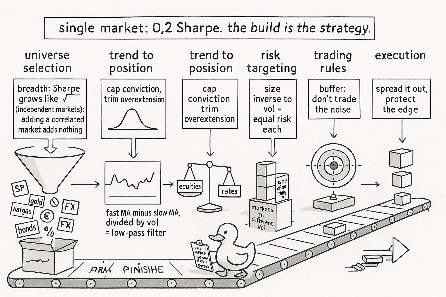
A trend follower is 0.2 Sharpe on one market; the build is the strategy. Walk all seven stages: universe breadth, vol-normalized crossover, capped sizing, sector balance, inverse-vol risk, and buffered execution.
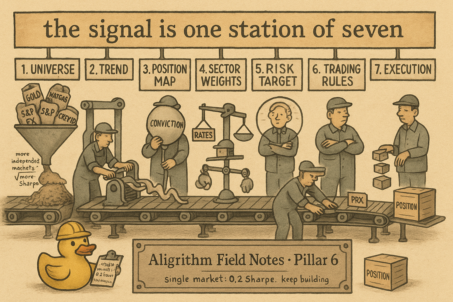
Trend following is the most straightforward systematic strategy to describe: buy what has been going up, sell what has been going down. It is also a roughly 0.2-Sharpe strategy on any single market, which is to say a bad one, and the gap between that description and a fund that runs billions is entirely construction. The signal is the part everyone fixates on and the part that matters least. The work lives in the six components wrapped around it. Walk them in order and the strategy assembles like a machine where every part earns its place.
The pipeline has seven stages: universe selection, trend detection, mapping trend strength to a target position, sector and asset-class weights, portfolio risk targeting, trading rules, and execution. None is optional, and the order is not arbitrary.
Universe selection: breadth is the whole game
Single-market trend following posts about 0.2 Sharpe, which nobody would trade. The strategy is rescued by breadth, and breadth scales in a specific way.
$$ \text{Sharpe}_{\text{portfolio}} \;\propto\; \sqrt{\text{breadth}} $$ $$ \text{breadth} = \text{number of independent markets you trade} $$
Read that as: the portfolio Sharpe grows with the square root of the number of genuinely independent markets you run the strategy across. The word doing the work is independent. If you already trade S&P 500 and Nasdaq futures, adding Dow futures buys you almost nothing, because the Dow is the same bet you already hold, and the square-root law counts independent markets, not tickers. Add natural gas instead and you add a market whose trends fire on their own schedule, and the breadth count actually rises. This is the old article "The Death of the Single-System Trader" applied to markets rather than systems: correlated components give you almost no diversification, so the count that matters is the effective independent count, not the raw one.
A typical futures trend follower trades 60 to 80 markets across the major exchanges. A larger and more sophisticated shop pushes into 300 to 400, reaching for niche futures like power, freight, and crypto, plus FX forwards, rate swaps, and CDS indices, because each genuinely different market adds another independent draw to the average. Expanding the universe this way can lift the strategy's Sharpe by a factor of one and a half to two, which is a larger improvement than any amount of signal tuning will ever give you. The universe is the highest-leverage decision in the build, and it comes first for that reason.
Trend detection: a vol-normalized low-pass filter
The signal matters less than its reputation, because it is usually obvious whether a market is trending, and the only job is to capture that quantitatively without overfitting. The standard tool is a moving-average crossover: a fast moving average of log price minus a slow one, normalized by volatility.
$$ \text{raw trend} \;=\; \text{MA}_{\text{fast}}(\log P) \;-\; \text{MA}_{\text{slow}}(\log P) $$ $$ \text{signal} \;=\; \frac{\text{raw trend}}{\sigma} $$
Read that as: take a fast and a slow moving average of the log price, subtract to get the raw trend, then divide by the market's volatility so the signal is in risk units and comparable across a fast market and a slow one. The vol normalization is the same logic as the old article "Why ATR Normalization Is More Than a Volatility Trick": without it, a high-vol market dominates the book for no good reason. The crossover survives because it is simple, hard to overfit, and acts as a low-pass filter, stripping the high-frequency return noise and leaving the slow drift, which is exactly the thing the old article "Efficiency Ratio Explained for Traders" measures from the other direction. Trend followers typically detect on horizons from one month to one year, centered around three to six months. Shorter than that and you are a different, smaller business; longer than a year is rare.
Mapping trend to position: cap the conviction
A raw signal of arbitrary size is not a position. You pass it through a function that maps trend strength to a target risk allocation, and the point of the function is to stop you from building forever as the trend gets stronger. Two shapes are common.
$$ \text{position} = \text{sigmoid}(\text{signal}) \qquad\text{or}\qquad \text{position} = \text{signal}\cdot e^{-\,\text{signal}^2} $$
Read that as: either a sigmoid, which saturates so the position flattens out at a maximum once the trend is strong enough, or a function like signal times e to the minus signal-squared, which rises, peaks, then actually shrinks the position for extreme signal values. The second shape encodes overextension: a trend that has run absurdly far is more likely to snap back, so you trim rather than press. Both refuse to let a single roaring market take over the whole risk budget, which is the same discipline as capping any one bet, and the choice between them is a view on whether very strong trends keep paying or tend to reverse.
There is a tempting addition here that deserves a skeptical flag. You can add a long bias to this function for markets that drift up on average, equities, credit, fixed income, and it does tend to improve backtested Sharpe. It also quietly guts the best property the strategy has, its ability to make money in an equity or bond bear market, because you have bolted a permanent long onto a strategy whose whole selling point is that it does not care which way the market goes. Many managers do it anyway for the Sharpe bump. The honest cost is that you are no longer running a pure trend follower, you are running a trend follower plus a hidden long, and the hidden long is the part that will hurt you in the crisis you bought the strategy to survive.
Sector and asset-class weights: undo the accidental tilt
Equal-weighting every market sounds neutral and is not. If you trade twice as many equity-index futures as rate futures, equal weighting leaves you structurally overweight equities, so a single bad month for stocks dominates a portfolio that was supposed to be balanced. Fix it by weighting up the under-represented sector, doubling the rate positions in that example, so risk is balanced across asset classes rather than across ticker counts. The same correction applies within a sector: commodity markets are less correlated with each other than rate markets are, so a basket of commodities carries more independent breadth per market than a basket of rates, and the weights should reflect that. This stage is housekeeping, and skipping it means your carefully chosen universe quietly collapses back into a concentrated bet.
Portfolio risk targeting: size inverse to volatility
Now size the positions. The standard rule makes each market's position inversely proportional to a forecast of that market's volatility.
$$ \text{size}_i \;\propto\; \frac{\text{target position}_i}{\sigma_i^{\text{forecast}}} $$ $$ \sigma_i^{\text{forecast}} \;=\; w\,\sigma_i^{\text{long-run}} \;+\; (1-w)\,\sigma_i^{\text{short-run}} $$
Read the top line as: for a given trend strength, you size the position down in proportion to how volatile the market is, so every market contributes about the same amount of risk to the book and no single one can dominate. That equal-risk-contribution idea is the old article "Why Volatility-Adjusted Position Sizing Matters" applied across a whole portfolio. The volatility forecast in the denominator can be as elaborate as you like, but the bottom line is the practical truth: you capture most of the benefit with a simple blend of a long-run volatility estimated over years and a short-run realized volatility over the last 30 to 60 days. The long-run term keeps the estimate steady, the short-run term lets it react when a market wakes up, and the blend is robust precisely because it is not trying to be clever.
Trading rules and execution: stop trading the noise
The last two stages are where a clean backtest meets its costs. A naive implementation re-sizes to the exact target every day, and the target jiggles constantly because the volatility forecast and the signal both wobble, so you pay round-trip costs on changes that carry no information. The fix is a buffer: leave the position alone while it sits inside a no-trade band around the target, and only trade when it drifts outside the band. That converts a stream of tiny noise trades into occasional meaningful ones, which is the cost-side version of the same noise problem the old article "Signal Averaging: Killing Noise with Redundant Alphas" attacks on the signal side. Execution then spreads the resulting trades over time to keep market impact small, because a trend follower's edge is measured in fractions of a percent and clumsy execution gives all of it back. These stages produce no alpha. They decide how much of the alpha from the first five stages actually reaches your account.
Visualizing the pipeline
KEY POINTS
- Trend following on a single market is about 0.2 Sharpe. Everything good about it comes from the six components wrapped around the signal, not the signal.
- Universe selection comes first and matters most. Sharpe grows like the square root of the number of independent markets, so adding a correlated market buys nothing and adding an uncorrelated one buys a lot. Expanding the universe can lift Sharpe one and a half to two times.
- The trend signal is a fast minus slow moving average of log price, normalized by volatility. It is a low-pass filter, simple and hard to overfit, run on one-month to one-year horizons centered on three to six months.
- Map trend strength to a target through a saturating or overextension-trimming function so no single roaring market eats the risk budget. Adding a long bias for equities and bonds lifts backtested Sharpe but destroys the strategy's bear-market hedge; that is a real cost, not a free lunch.
- Weight sectors and asset classes to undo the accidental tilt from trading more markets in one sector than another. Equal-weighting tickers is not equal-weighting risk.
- Size positions inversely to a volatility forecast so every market contributes equal risk. A simple blend of long-run and 30 to 60 day realized vol captures most of the benefit.
- Trading rules and execution decide how much alpha survives. Use a no-trade buffer to stop trading the noise, and spread execution to keep impact small. These stages make no alpha; they protect it.