The trader running one system is one regime change away from being broke. The question is not whether the system will die. The question is when, and what will be left running when it does.

Every working rule decays. The market structure that produced the edge changes. Participants rotate. Volatility regimes shift. The rule that delivered Sharpe 1.4 for three years stops delivering anything for the next three. The trader who built a career on that rule, with no second rule running in parallel, has a career that lasts as long as the rule does.

A system death is quiet. The equity curve does not collapse on a single day. It grinds sideways for nine months, the trader explains it as "a normal drawdown," the curve grinds sideways for another nine months, the trader starts re-optimizing parameters, the curve grinds sideways for another year, and at some point the trader runs out of capital, conviction, or both. The system did not blow up. It stopped delivering, with nothing else to take up the slack.

The math of why one is not enough

Take a single system with Sharpe ratio S and volatility σ. Now imagine running N such systems together, each with the same Sharpe and volatility, all scaled to equal capital weight.

The portfolio volatility depends on the correlation between systems.

In plain words. The numerator is the average pairwise covariance, scaled by the number of pairs in the basket. The denominator is the number of systems. As N grows, the average pairwise correlation ρ drives whether portfolio volatility falls or stays the same.

Three cases.

If ρ = 0 (systems are independent), σ_p = σ / √N. Five independent systems have 0.45σ volatility. Twenty have 0.22σ.

If ρ = 0.5 (systems are moderately related), σ_p = σ √((1 + 0.5(N-1))/N). Five such systems have 0.77σ volatility. Twenty have 0.72σ. The diversification benefit stalls around 0.71σ as N grows, because √ρ is a floor that no amount of additional systems can break through.

If ρ = 1 (systems are identical), σ_p = σ. No diversification at all. Twenty copies of the same system is one system at full risk.

The portfolio Sharpe ratio inverts the volatility result.

Same three cases. Five independent systems produce portfolio Sharpe of S × √5 ≈ 2.24 × S. Five moderately correlated systems produce S × √(5/3) ≈ 1.29 × S. Five identical systems produce S × 1 = S.

The takeaway: adding systems that are independent of each other doubles or triples the achievable Sharpe ratio. Adding systems that are correlated does little. The diversification benefit is not in having "many systems." It is in having many independent systems. Running ten different parameter variants of the same EMA crossover is one system in costume.

The decay case

Every rule decays. The decay timing is not synchronized across rules that capture different market behaviors.

A trend-following rule on commodity futures decays when commodity volatility collapses. A mean-reversion rule on equity intraday decays when intraday liquidity structure shifts. A carry rule on FX decays when rate differentials compress. These are different events. They happen at different times. They do not all happen in the same year.

A trader running five uncorrelated systems is running five independent decay timers. The probability that all five timers fire within the same 12-month window is the product of the individual probabilities. If each system has a 20% chance of entering terminal decay in a given year, the probability that all five enter terminal decay in the same year is 0.2^5 = 0.00032, or 1 in 3,125. The probability that at least one continues to work is 1 − 0.00032 = 99.97%.

A trader running one system has a 20% chance of entering terminal decay in a given year, full stop. Over five years, the probability of at least one terminal decay event is 1 − 0.8^5 = 67%. The single-system trader is more likely than not to be in terminal decay within five years. The five-system trader is statistically certain to have at least one working system in the same window.

This is a counting argument. The single-system trader is making a bet that the next regime change happens after they retire. That bet has a known and unfavorable distribution.

The behavioral case

Equity-curve psychology compounds the structural problem.

A single-system trader watches one curve. The curve has the natural drawdown distribution of one strategy. A deep drawdown on that curve gives the trader no other curve to compare it to. The question becomes "is my system dead, or is this a normal drawdown?" The trader cannot tell. The information needed to answer the question is the behavior of similar but uncorrelated systems, which the trader does not run.

The result is that the single-system trader makes the kill decision at the wrong time. They wait too long to switch off a dying system, because the drawdown looks normal until it is too deep. Or they switch off a healthy system during a normal drawdown, because the drawdown feels worse than the trader expected.

A portfolio trader has the comparison signal built in. If four systems are flat or up and one is in deep drawdown, the diagnosis is "that system is breaking, the others are not." If all five are in drawdown together, the diagnosis is "the regime has changed in a way that affects all of them, this is a portfolio-level event, not a system-level one." Different diagnoses, different responses.

The portfolio also stabilizes the equity curve emotionally. A drawdown of 25% on a single system looks like the end of the trader's career. A drawdown of 6% on a portfolio of five uncorrelated systems, where one component is down 25% but the others are flat, looks like a routine quarter. The same underlying single-system loss is psychologically survivable inside the portfolio and unsurvivable outside it.

Real diversification, not parameter cosplay

The math requires the systems to differ in structure. Variants of the same idea do not count.

Different rule families. Trend-following, mean-reversion, carry, volatility-targeting, breakout, momentum, lead-lag. Each family captures a different market behavior. Mixing within a family gives correlated returns. Mixing across families gives independent returns.

Different instruments. The same rule run on FX, equity indices, commodities, and rates is four exposures to different macro factors, which is closer to four systems than one. Even a rule family with high correlation within an asset class (for example trend following on equity indices) becomes uncorrelated when run on different asset classes.

Different timeframes. A trend system on daily bars and a trend system on 5-minute bars trade different things. The slow system captures macro regime shifts. The fast system captures intraday flow imbalances. Their correlations sit below 0.3 even though both are "trend following."

Different signal sources. Price-based signals, volume-based signals, volatility-based signals, cross-asset signals, fundamental signals. Each source has different decay drivers. A volume-based microstructure rule decays when market structure changes. A volatility-targeting rule decays when the volatility regime shifts. They do not die at the same time.

The diversification axis to avoid is parameter variation. Running the same EMA crossover with lookback windows of 10, 20, 30, and 40 bars is not four systems. It is one system run with overlapping settings. The correlation between variants is often 0.85 or higher. The portfolio Sharpe improvement from such "diversification" is small.

Picking the right N

Diversification benefit follows a sharp diminishing-returns curve. The first additional system cuts portfolio volatility most. Each subsequent system contributes less.

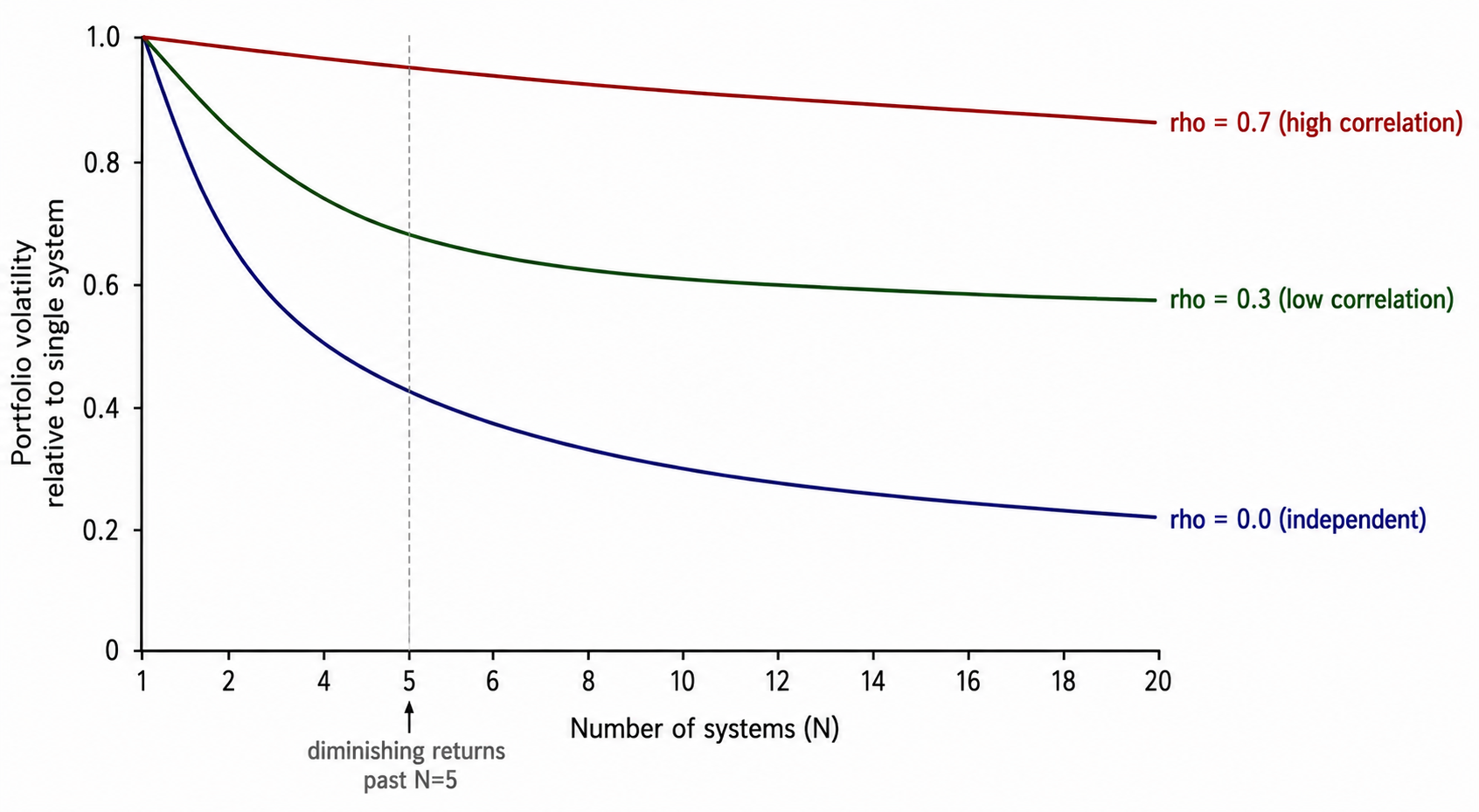
The visual shows the practical answer. With independent systems, going from 1 to 5 cuts volatility by more than half. Going from 5 to 20 cuts it by another half. Going from 20 to 100 cuts it by another half. Each cut requires four times the number of systems.

Operationally, 4 to 6 uncorrelated systems is the sweet spot for retail and small-fund traders. Below 4, the math has not delivered enough benefit. Above 6, the operational complexity (monitoring, capital allocation, kill-switch management, infrastructure) starts to outweigh the marginal diversification gain. Institutions with operational teams push the number higher. Solo traders should not.

The other constraint is capacity. Each system has a capacity limit beyond which slippage and market impact eat the edge. Running 30 systems at $1 million per system requires $30 million in capital, which most readers do not have. The diversification benefit caps out wherever the trader's capital runs out.

The standard death arc

The path is familiar enough to write down by year.

Year 1: trader builds a system. Backtest looks great. Live deployment in year 2 confirms the backtest in the first few quarters. Trader feels validated. Trader scales up position size.

Year 3: trader is at full position size. The system produces a year that matches backtest expectations. Trader concludes the system "is working."

Year 4: a quiet shift happens in the market structure the system was fitted to. The system stops producing the expected returns. The equity curve enters a sideways grind. Trader interprets this as a normal drawdown and waits.

Year 5: the grind continues. Trader starts re-optimizing parameters to recover the backtest performance. New parameters help for a month. Then the grind returns. Trader re-optimizes again.

Year 6: the account is well below its peak. Trader exits the market either out of capital or out of conviction. Trader either quits trading or starts the process over with a new system, having lost five years of capital and time.

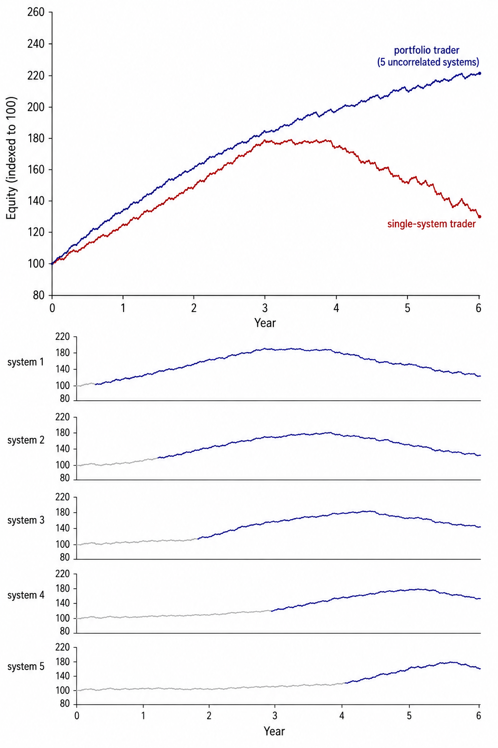
The portfolio trader following the same career path has component systems entering and leaving the rotation throughout. By the time the original system dies in year 4, two replacement systems have already been added in years 2 and 3. The portfolio kept producing returns while individual components died and were replaced. The career length is open-ended.

The single-system trader was never wrong about the original rule. The original rule worked. The structural error was running it without anything else alongside.

KEY POINTS

• Every working rule decays. The question is when, not whether. A trader with one rule has a career as long as the rule.
• Portfolio volatility for N equal-weight systems with average pairwise correlation ρ is σ × √((1 + (N-1)ρ) / N). Independent systems compound the Sharpe ratio by √N.
• Five independent systems produce portfolio Sharpe of around 2.24x the single-system Sharpe. Five identical systems produce no benefit at all.
• Different rule families, different instruments, different timeframes, and different signal sources are sources of real diversification. Different parameter values on the same rule are not.
• Running uncorrelated systems gives the trader an independent comparison signal for diagnosing decay. The single-system trader has no comparison and makes the kill decision at the wrong time.
• Diminishing returns set in around N = 5 for independent systems and around N = 3 for moderately correlated systems. Adding more systems beyond that point trades operational complexity for marginal diversification.
• The standard single-system death arc takes 5 to 6 years from initial deployment to exit. The portfolio trader replaces components on a rolling basis and avoids the terminal event.