6. Portfolio Construction & System Death October 31, 2026 15 min

6.60 Regime Bake-Off: Five Methods, Do They Agree on the Breaks?

Regime breaks on one price path: a piecewise-linear knee and a volatility Markov chain mark different dates. Write down which break you meant before you trade it.

Five rules for where a regime changed, fitted to one 480-day price, do not return one calendar. The path is planted. Drift changes on days 120, 280, and 420. Volatility changes on days 200 and 340. Each break moves only one of those two, and the days are numbered from zero. The piecewise-linear knee in the old article "Piecewise-Linear Regime Identification (Interpretable, No Black Box)" puts knots on days 129 and 270. The high-volatility rule in the old article "Regime-Switching That Works, Factors That Don't (MS-GARCH)" steps into the high-volatility state on day 201 and marks none of the drift breaks. Treat the path as a Rorschach blot: each method circles the feature it was built to see.

Two knots, and the third drift break never gets one

Steiner's note fits a connected straight line to an index level. The slope is constant until a knot, the level does not jump, and the change in slope at knot j is one coefficient. With the sample running over days t = 0, 1, ..., 479 and the positive-part hinge (x)+ equal to max(0, x):

$$ y_t = \beta_0 + \beta_1 t + \sum_{j=1}^{K} \beta_{j+1}\,(t - \tau_j)_+ $$ $$ \text{slope after knot } m = \beta_1 + \sum_{j=1}^{m} \beta_{j+1} $$

Before the first knot the slope is β1. Each later coefficient is the kink at that knot, so the slope on a segment is the opening slope plus every kink that has already fired. Continuity is free: the hinge is zero at its own knot, so the left-hand and right-hand levels match. On this path the knee, computed below, picks K = 2. The fitted coefficients are β0 = 95.953686, β1 = 0.018783, β2 = −0.359422 at day 129, and β3 = 0.354067 at day 270.

Day 129 is the first kink. The fitted level is 95.953686 + 0.018783 × 129 = 98.3767. The slope changes by −0.359422, from 0.018783 to −0.340639 price points a day. Over the 141 days from day 129 to day 270 that slope takes off 141 × 0.340639 = 48.0301, and the fitted level on day 270 is 98.3767 − 48.0301 = 50.3466. The second kink adds 0.354067 and the slope for the rest of the sample is −0.340639 + 0.354067 = 0.013428. The line falls through the crash and then lies almost flat. It does not bend again at day 420.

Steiner picks the knot count off the R-squared curve. He plots in-sample R-squared against K and takes the knee, the interior point farthest from the straight line that joins K = 0 to K max. R-squared here, with each segment forced to at least 20 days (wider than the note's typical 2 to 10 observations, so a knot cannot sit on a one-week blip), runs

0.8142, 0.8991, 0.9772, 0.9870, 0.9884, 0.9916, 0.9922

for K = 0 through 6. The chord from (0, 0.8142) to (6, 0.9922) has direction v = (6, 0.1780).

$$ d_k = \frac{\lvert v_x (R^2(k) - R^2(0)) - v_y \, k \rvert}{\lVert v \rVert} $$

The distance is the absolute size of the two-dimensional cross product of the chord and the vector from the left endpoint to the point (k, R-squared of k), divided by the length of the chord. For K = 2 the rise in R-squared is 0.9772 − 0.8142 = 0.1630. The cross product is 6 × 0.1630 − 0.1780 × 2 = 0.622. The chord length is the square root of 36 + 0.1780 squared, which is 6.0026. The distance is 0.622 / 6.0026 = 0.1036. The same arithmetic at K = 1, 3, 4, and 5 gives 0.055, 0.084, 0.056, and 0.029. The knee is K = 2.

Those two knots sit 9 days after the first planted drift break and 10 days before the second. The third drift break, day 420, gets nothing. Both volatility breaks get nothing. The old article already showed that Steiner's own Swiss Leaders ladder, an in-sample R-squared of 0.954 at fifteen breakpoints, is matched or beaten by a driftless random walk of the same length. A high R-squared is what a flexible line does to one path. The knee tells you where the line stopped spending knots. It does not tell you that a volatility regime flipped.

Theta of 0.04 confirms the turn, and twenty other days

The old article "State-Dependent (In)Efficiency: Meta-Learning a Directional-Change Threshold" throws out the calendar. A directional-change confirmation fires when price reverses by a fraction theta from the last extreme. In an upswing you track the running high. In a downswing you track the running low.

$$ P_c \le P_{\mathrm{high}} \times (1 - \theta) \qquad P_c \ge P_{\mathrm{low}} \times (1 + \theta) $$

The left inequality confirms a downtrend. The right one confirms an uptrend. Pc is the price now, and the extreme is the high or low since the previous confirmation. On this path the running high on day 15 is 100.86. At theta of 0.04 the downtrend line is 100.86 × 0.96 = 96.83. Day 20 prints 96.06, which is through that line, so a downtrend is confirmed. The first planted drift break is day 120. The first confirmation is noise, a hundred days early.

Count the confirmations. Theta of 0.01 fires 100 times, theta of 0.02 fires 49 times, and theta of 0.04 fires 23 times. The confirmation nearest each planted drift break is within eight days at all three settings: at theta of 0.04 the lags are +4 days, −3 days, and −2 days. The same coarse theta also confirms inside both volatility breaks, on days 203 and 207 and again on days 334 and 339, because a 2.5 percent daily volatility produces 4 percent reversals while the drift is unchanged. Twenty-three dates name turns.

Barak, Razmi, and Mousavi do not stop at one theta. A classifier picks tomorrow's theta from the set {0.01, 0.02, 0.04} using today's features, and the label it trains on is whichever theta made the most money that day. Their SHAP plots say the small theta is chosen when the price z-score is high and Ethereum exchange netflow is positive, an overbought book with coins moving onto exchanges, and the large theta is chosen when positions are already long and netflow is negative. The split is a mean-reversion state against a trend state. I do not have their on-chain panel, so the days their classifier would have switched theta are absent from the figure. The three static counts already show the problem. Move from theta of 0.01 to theta of 0.04 and the list shrinks from 100 dates to 23, while the nearest hit on a real drift break stays inside eight days.

High volatility starts the day the probability clears one half

De la Torre-Torres, Álvarez-García, and del Río-Rama trade lumber with one inequality. If the probability of the high-volatility state next period is above 0.50, hold Treasury bills. If it is at or below 0.50, hold the lumber future. The printed forecast multiplies a transition matrix by a probability vector whose first entry is indexed at t+1 and whose last entry is indexed at t. Those cannot be the components of one vector. I keep their trading rule, which is the one-step probability, and I do not use the mis-indexed display. With plow and phi the filtered probabilities of the low and high states given returns through today, and P(high | low) and P(high | high) the two transition probabilities into the high state:

$$ \xi_{\mathrm{high},\, t+1} = P(\mathrm{high} \mid \mathrm{low})\, p_{\mathrm{low}, t} + P(\mathrm{high} \mid \mathrm{high})\, p_{\mathrm{high}, t} $$

You are mixing today's filtered weights with the chance each state moves into high volatility tomorrow. On this path the filter is a two-state Gaussian with one shared mean and a separate volatility in each state. That is their time-fixed variance engine. The exponential GARCH engine is the one that made the lumber profit. The fitted volatilities are 0.0069 and 0.0246, against planted levels of about 0.008 and 0.025. The high state stays high with probability 0.9926. The low state stays low with probability 0.9969.

On day 200 the filtered weight is 0.0271 on the low state and 0.9729 on the high state. The one-step high-volatility probability for day 201 is 0.0271 × 0.0031 + 0.9729 × 0.9926 = 0.000084 + 0.9657 = 0.9658. That clears 0.50, so the rule calls day 201 a high-volatility day, one day after the planted jump. It steps back out on day 346, six days after the planted drop on day 340, with two one-day holes on days 261 and 300 where the probability dips under 0.50 and comes straight back. None of the three drift breaks is crossed. The parameters are fit on the whole sample, so the two volatilities know the future even though the day-by-day probability is filtered forward. The percentile method has the same lookahead in its cutoffs. Here the lookahead sits in the two volatilities.

The lumber paper's equation (6) is why I did not mark these dates with a GARCH recursion. They describe a symmetric GARCH and then print a linear filter on the raw residual and on the volatility, plus a disturbance. Specialized to one lag, with the disturbance set to zero for the arithmetic:

$$ \hat\sigma_t = \alpha + \beta \, \epsilon_{t-1} + \gamma \, \hat\sigma_{t-1} $$

Plug in α = 0.002, β = 0.10, γ = 0.80, yesterday's volatility 0.02, and a residual of −0.25. The update is 0.002 + 0.10 × (−0.25) + 0.80 × 0.02 = 0.002 − 0.025 + 0.016 = −0.007. A volatility cannot be negative. Bollerslev squares the shock and the variance. Equation (6) does neither. I keep their expression and treat the display as likely wrong. The dates above use the time-fixed engine on purpose. On lumber, that engine with a Gaussian likelihood lost 52.94 percent. The asymmetric exponential GARCH with a generalized-error likelihood, which they also do not print as a formula, made 158.33 percent against a buy-and-hold accumulated return of 7.13 percent over 1,022 weeks. Swap the variance equation and the sell dates move. The 0.50 line only reads out a probability the variance engine has already shaped.

The 20th percentile is a line drawn with the whole sample

The old article "Volatility Clustering in Bitcoin: Regime Persistence as a Forecast" builds a three-state chain on rolling log-volatility. Borrego Roldán computes a trailing standard deviation of simple price ratios, takes the log, and cuts the full sample at the 20th and 80th percentiles. Those two cutoffs were chosen arbitrarily, and they use the whole history, including the future. Low is below the 20th percentile. Medium is between the cutoffs. High is above the 80th.

$$ s_t = \begin{cases} \mathrm{low} & \text{if } \ln \sigma_t < q_{0.20} \\ \mathrm{high} & \text{if } \ln \sigma_t > q_{0.80} \\ \mathrm{medium} & \text{otherwise} \end{cases} $$

σt is the standard deviation of the last 20 daily returns, and the two q values are percentiles of ln σ over every day the window is full. On this path those percentiles are −5.0656 and −3.8341, which are rolling volatilities of 0.63 percent and 2.16 percent. The quiet regimes, planted near 0.8 percent and 0.7 percent, sit in the middle bucket unless a stretch dips under 0.63 percent. The noisy regime, planted at 2.5 percent, sits above 2.16 percent, so it can register as high. The chain enters the high state on day 209, nine days after the planted jump, having stepped from low to medium on day 200 itself. It then flips between medium and high twenty times by day 349. There are 43 state changes in the sample. A hard threshold on a wiggling rolling volatility is a flicker machine.

The paper's own chain is stickier than this path, and the stickiness is the object worth computing. On the 7-period daily Bitcoin matrix the low state stays low with probability 0.8167, goes to medium with probability 0.1787, and goes to high with probability 0.0045. The row sums to 0.9999, so the last 0.0001 is rounding and the source may have truncated a digit. Using the printed stay probability:

$$ \text{expected run} = \frac{1}{1 - 0.8167} = 5.46 \text{ days} $$

A state that exits with probability 0.1833 lasts 1 / 0.1833 = 5.46 days on average. The other two stay probabilities on that same matrix are 0.8875 and 0.8371. The medium state lasts 1 / 0.1125 = 8.89 days, and the high state lasts 1 / 0.1629 = 6.14 days. The paper's shortest persistence anywhere in the study is this 0.8167, and most of the other matrices sit above 0.9. In the high state they report a one-standard-deviation move of about 9 percent inside 48 hours. In the low state, one standard deviation is often under 5 percent even out to seven days. The number forecasts the size of the next move given the bucket. The drift break is a separate date, and the bucket edges were drawn with the sample you are trying to label.

The l1 penalty bends in different places

The old article "Fair Value as an Adaptive Low-Pass Filter: LAFO for Mean Reversion" treats fair value as the output of a low-pass filter. The local-average filtering objective, LAFO, scores the filtered line by the squared average residual inside a window of length K. At K = 1 the window is one bar and LAFO is mean squared error. At K equal to the whole sample the objective only sees the average residual, and a flat line at the mean drives it to zero whenever the residuals sum to zero. Residuals of +3, 0, and −3 have a mean squared error of (9 + 0 + 9) / 3 = 6, and a LAFO of 0 when the window is the whole sample. Xu, Firoozye, Koukorinis, Treleaven, and Zhu then add a penalty that decides the shape of the line. The penalty that places slope breaks is the l1 trend filter, an absolute penalty on second differences. With K = 1, so the data term is the ordinary squared error and the knots come from the penalty:

$$ \mathcal{L} = \frac{1}{T}\sum_{t=1}^{T}(y_t - \hat y_t)^2 + \lambda \sum_{t=3}^{T} \lvert \hat y_t - 2\hat y_{t-1} + \hat y_{t-2} \rvert $$

The second difference is the change in slope. The absolute penalty drives most of those changes to zero and leaves a few kinks, which is a piecewise-linear fair value. Three consecutive fitted values 100, 101, and 100.5 have first differences +1 and −0.5, so a total-variation penalty on levels would charge 1.5. The second difference is 100.5 − 2 × 101 + 100 = −1.5, so the l1 trend penalty also charges 1.5 on that one kink, and charges nothing on a stretch whose slope is constant. Lambda is how hard you press. I set it to 2.15 because that was the grid point whose kink count came closest to the knee's two knots. The closest the grid came was three kinks, on days 108, 207, and 260.

Day 108 is 21 days from the piecewise knot on day 129. Day 260 is 10 days from the piecewise knot on day 270. Day 207 is seven days after the volatility break and has no piecewise partner, because the knee was rationed to two knots and spent them on the crash turns. Two slope methods, matched as nearly as the penalty grid allowed on how many kinks they may spend, still disagree on where the slope changed. Both miss day 420. The planted drift from that day is 0.16 percent a day for 60 days, about 10 percent if the noise averages out. The realized price goes from 53.02 on day 419 to 50.90 on day 479. The noise ate the drift, and a knee with only two knots was never going to circle a break the path itself does not show.

Their trading demo on two-minute S&P 500 data, two months, 3 basis points of cost, is a separate claim and a weak one. The two-layer network posts an in-sample Sharpe ratio of 11.05. The exponential moving average of length 10 posts −18.27. The authors call the exercise methodological and say they did not calibrate it out of sample. A Sharpe ratio of 11 on two-minute bars is a stress test of credulity. The penalty, not that Sharpe ratio, is the part that belongs in a break date.

The dates do not line up

Look at the red piecewise line. It bends after the first dashed drift break and again before the second, and it stays straight through both dotted volatility breaks and through the last dashed drift break. The blue line is the l1 trend filter. The rug underneath is every date the five rules marked.

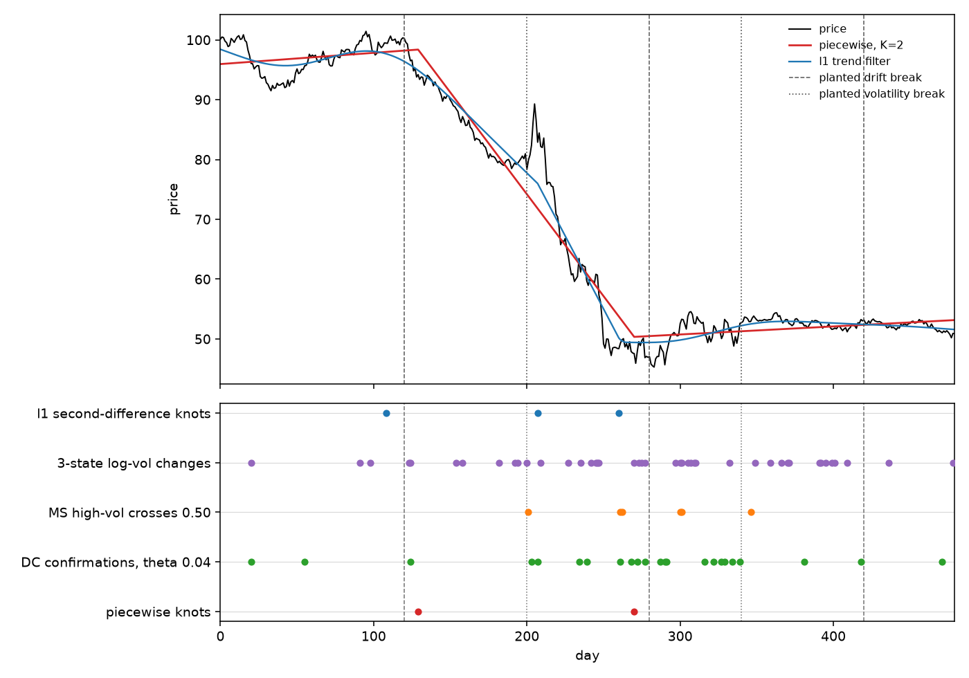
Planted 480-day price with a two-knot piecewise fit and an l1 trend filter, dashed lines at the three drift breaks and dotted lines at the two volatility breaks, and a rug of piecewise knots, 4 percent directional-change confirmations, Markov-switching 0.50 crosses, three-state log-volatility changes, and l1 knots

Three numbers. The knee's R-squared is 0.98, with knots on days 129 and 270 and nothing on day 420. The one-step high-volatility probability is 0.97 on day 201, and that rule marks none of the drift breaks. Theta of 0.04 confirms 23 times. The rest of the published scoreboard is one sentence: on lumber the generalized-error exponential GARCH book made 158.33 percent while the Gaussian time-fixed book lost 52.94 percent, against buy-and-hold at 7.13 percent; the crypto meta-learner posts a Sharpe ratio of 1.34 against 0.59 for the best static theta, gross of fees, with a Ledoit-Wolf bootstrap p-value of 0.008; the two-minute network's Sharpe ratio of 11.05 is the in-sample demo above.

A ten-day window makes some of these dates look like matches. The piecewise knot on day 270 sits near a cluster of percentile flickers and near one of the one-day holes in the Markov-switching filter. Those neighbors are volatility chatter inside a noisy decline. The knot is trying to mark the drift change on day 280. Sharing a neighborhood is not sharing a question. The Rorschach blot did not get clearer because two pencils landed an inch apart.

Write the question down before you size anything

At the desk you write one sentence before you look at a date. Either you want the day the drift changed, or you want the day the volatility changed. The hinge and the l1 penalty answer the first, and they still missed day 420 and disagreed with each other by three weeks on the first kink. The 0.50 filter and the percentile chain answer the second, and the chain flickered 43 times while the filter was late by a day on the way in and six days on the way out. A directional-change confirmation answers a third question, where price reversed by theta, and the meta-learner's theta switch answers a fourth, which mesh makes money tomorrow. I am against averaging those four answers into one regime score and then sizing a book off it.

None of the dates on the figure were tradable on the day they happened. The knots, the percentile cutoffs, and the two Gaussian volatilities all see the full 480 days. An expanding window will move the knot, and it will move the 20th percentile, and the state you thought you were in last month will be relabeled. The Bitcoin low state lasts about 5.46 days once you are in it, so a hedge that waits for the chain to step out is late by that order even before the lookahead in the cutoffs. The crypto strategy is gross of fees; the old article already ran the static theta of 0.01 down to a profit factor of about 1 at 16 basis points, before funding. This path charges no spread at all. If two methods that were built for the same question land inside ten days, you have a candidate date. Otherwise the date stays a pencil mark on the blot.

KEY POINTS

Stop the piecewise fit at the knee. On this path the knee is two knots, days 129 and 270, at an R-squared of 0.98, and the drift break on day 420 is unmarked.
Do not read a directional-change confirmation as a volatility regime. Theta of 0.04 confirms 23 times, close to all three drift breaks and inside both volatility breaks.
Flip the book when the one-step high-volatility probability crosses 0.50. Here that entry is day 201, and the rule marks none of the drift breaks.
Treat a full-sample 20th percentile as lookahead. The 7-day Bitcoin low state stays put with probability 0.8167, an expected run of 5.46 days, and the row as printed sums to 0.9999.
Do not separate the lumber date from the variance engine. The Gaussian time-fixed book lost 52.94 percent and the generalized-error exponential GARCH book made 158.33 percent, on the same 0.50 rule.

References

A note on AI. The ideas, research, analysis, and conclusions in this article are my own. I use AI tools to help with editing and wordsmithing, because English is not my first language, and I am not shy about that. AI-generated ideas and AI-assisted writing are not the same thing: the first is empty slop from a generic prompt, the second is a tool for communicating years of real research more clearly. Judge the work by its substance, not by whether software helped polish the prose.