5.67 State First, Event Second: L2 Liquidity-State Transitions in Crypto Futures

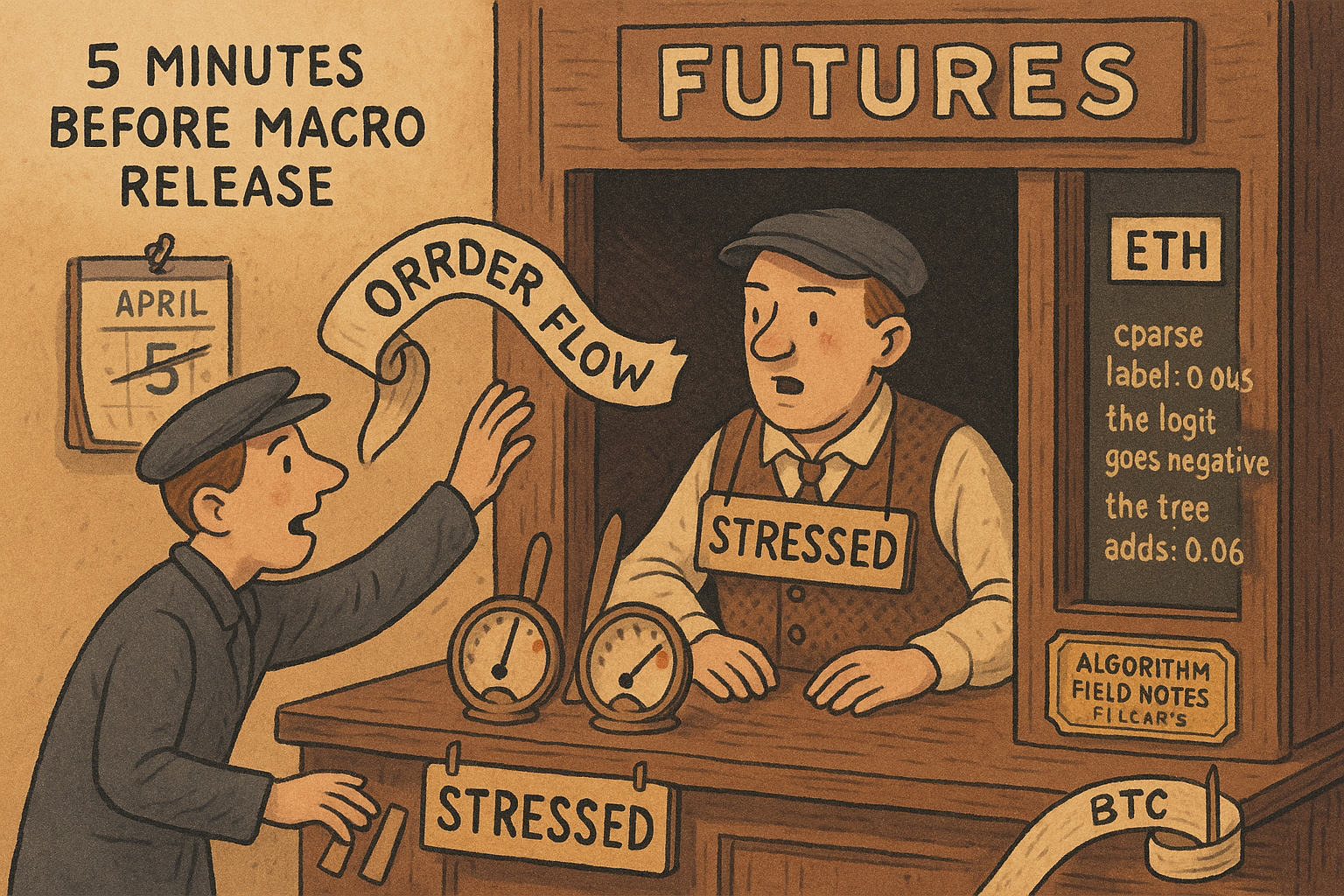
On the Binance BTCUSDT perpetual, the twenty best bids and asks in the five minutes before a scheduled macro release already put the book in one of three labels: calm, mixed, or stressed. Jeon builds the label from relative spread, top-20 depth, and top-20 imbalance, and he uses it to predict the same label after the release on BTCUSDT and ETHUSDT futures from 2023 into 2026. The pre-event label beats a model that knows only the label frequencies, by 0.045 at five minutes on the average of log-loss and Brier score. Log-loss is the average of minus the natural log of the probability on the label that printed. The Brier score is the average squared error of the three probabilities. He keeps a later feature only when that same average improves on the layer under it, on the same windows, and the release name stays out of the fit.

Two severe readings, and the book is stressed

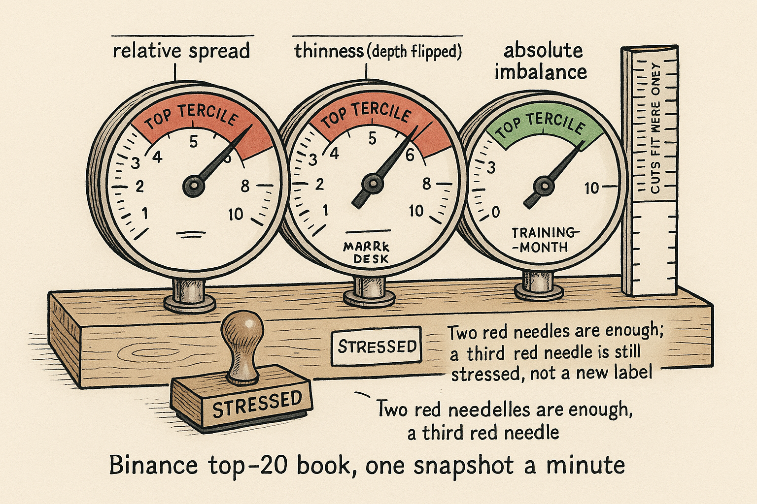
A minute is stressed when at least two of three oriented book measures sit in their top tercile. He estimates those cuts on the training months for that symbol only, then applies them to the held-out month. The count is capped at two, so a book that fails all three measures gets the same stressed label as a book that fails two.

$$ s = \frac{a - p_b}{m}, \qquad C = \min\left( \mathbf{1}\{s \ge \tau_s\} + \mathbf{1}\{-d \ge \tau_d\} + \mathbf{1}\{|u| \ge \tau_u\}, \; 2 \right) $$

C is how many ways the book looks illiquid, stopped at two. The relative spread s is the ask minus the bid, divided by the mid, so a one-dollar gap on a cheap contract does not outrank a one-dollar gap on a rich one. Depth d is the total size on the twenty best bids and the twenty best asks, and the minus sign puts the thin books into the top third. The imbalance u enters as an absolute value, so a bid-heavy book and an ask-heavy book are the same kind of severe. Each tau is the two-thirds quantile of that oriented series on the training months. C of 0 is calm, C of 1 is mixed, and C of 2 is stressed. Section 3.2 describes this cap and does not print the expression. The spread ratio and the usual size-imbalance ratio below are the operational reading of "relative spread" and "absolute imbalance," which he also does not print.

Take a mid of 100,000, a bid of 99,995, and an ask of 100,005. The gap is 10, and s is 10/100,000, which is 0.0001. On size, 800 contracts bid against 200 offered is an absolute imbalance of 600/1,000, which is 0.60, and 200 against 800 is the same 0.60. Negate three depths, 10, 100, and 1,000. You get −10, −100, and −1,000. The largest of those is −10, the thin book, and that is the one that can land in the top tercile.

Flags, not prices, finish the label. Spread severe, depth not, imbalance severe: the sum is 2, the cap leaves 2, and the minute is stressed. All three severe: the sum is 3, the cap returns 2, and the label does not get a fourth bin. One flag is mixed. None is calm. Across the scored windows the pre-event shares are about 0.21 calm, 0.54 mixed, and 0.25 stressed.

The release minute belongs to the label, not to the features

The target is the post-event label. Features stop at the release.

$$ Y_{i,h} = S^{\mathrm{post}}_{i,h}, \quad X_i \text{ from } [t - 5\,\mathrm{min},\, t), \quad Y_{i,h} \text{ from } [t,\, t + h), \quad h \in \{1, 5\} $$

For window i and horizon h, the thing you score is the liquidity label after the release. The pre-event vector aggregates the half-open five minutes ending at the release, so the release minute itself is not a feature. The label aggregates from the release up to, and not including, one minute later or five minutes later. He calls the five-minute combined label the primary specification and still reports both horizons. Same-country releases within sixty seconds are one window.

A release stamped 14:30:00 uses snapshots from 14:25:00 inclusive to 14:30:00 exclusive as the input, and the one-minute label uses 14:30:00 inclusive to 14:31:00 exclusive. The five-minute label runs to 14:35:00 exclusive. A second print from the same country at 14:30:40 shares that window instead of making a second row. He does not predict the sign of the return. The old article "Crypto Isn't Structurally Alien: Roll/VPIN/Amihud Predict Distribution Shifts" asks microstructure measures on Binance minute bars to call the sign of a later change in the return distribution. This target is the next book label.

The modeling universe is 47,513 windows at each horizon: 18,631 event windows (9,330 BTCUSDT, 9,301 ETHUSDT) and 28,882 matched non-event windows, from 9,773 scheduled events and 40 monthly folds, February 2023 through May 2026. BTC plus ETH is 9,330 + 9,301 = 18,631, and 18,631 + 28,882 = 47,513. Training months always precede the test month. The matched windows are shifted by a whole number of weeks so the hour of day and the weekday stay put. The United States is the largest region, 8,953 of the 18,631 event windows, which is 48 percent. High-importance and low-importance releases are near equal counts. Region, importance, the announced figure, and the surprise versus the forecast are on the calendar and out of the model. The book itself is a vendor snapshot of the twenty best levels, once a minute, over a sample where Binance also ships incremental depth. He chose the archive so the panel could run for years.

He prints, next to the construction, a five-minute joint improvement of 0.048 for the combined label over the marginal model, against 0.033 for the strongest single descriptor. Table 1 prints 0.045 for that same combined-label comparison on the held-out event windows. The text does not say why 0.048 and 0.045 differ. I use 0.045 for the scored table. The 0.048 may be another panel, or the source may be wrong. Either figure still sits above the single-descriptor 0.033.

Average the two scores, and make the next layer beat the average

He admits a layer only when it improves on the layer below it, on the same rows, out of sample.

$$ \mathrm{NLL}(M) = -\frac{1}{N}\sum_{i=1}^{N}\log p_M(Y_i \mid X_i), \qquad \Delta(M, B) = \mathrm{NLL}(B) - \mathrm{NLL}(M) $$

Negative log-likelihood, NLL, is the average natural-log penalty. A model that puts probability 0.10 on the label that printed pays −log(0.10), about 2.3, on that row. Delta is the baseline's NLL minus the candidate's NLL, so a positive delta means the candidate put more probability on what happened. The log in his equation is the natural log. A base-10 log would shrink every term by log(10) and would not match the arithmetic below.

$$ \mathrm{Brier}(M) = \frac{1}{N}\sum_{i=1}^{N}\sum_{k} \left(p_M(k \mid X_i) - \mathbf{1}\{Y_i = k\}\right)^2 $$

The inner sum runs over calm, mixed, and stressed. Each row contributes the squared distance between the probability vector and a one-hot label. He names the Brier score as the second proper score and does not print this sum. A proper score is one that is minimized when the probabilities you report are the ones you believe. The usual multiclass form is the sum over classes, which is what is written here. If his code averaged over the three classes instead, the Brier piece would be on a different scale, and the paper gives you no way to see which one he used.

$$ \Delta_{\mathrm{joint}}(M, B) = \frac{1}{2}\left(\Delta_{\mathrm{NLL}}(M, B) + \Delta_{\mathrm{Brier}}(M, B)\right) $$

The number in the table is the average of the two improvements. He describes that average and does not print it. For the coarse label at five minutes he prints an NLL gain of 0.061 and a Brier gain of 0.028. Half of 0.089 is 0.0445, and Table 1 prints 0.045. The same pair, an NLL gain of 0.061 and a Brier gain of 0.028, is what the note prints for the nonlinear model at one minute, and that cell is printed as 0.044. Identical rounded inputs, two reported averages. Keep both. The fourth decimal is where the source may have rounded one half up and the other half down, after the components were already rounded. The one-minute coarse-state pair does close: 0.046 and 0.022 average to the printed 0.034.

The marginal model is the training frequency of each label given the symbol and the horizon. No book. The state model is the training frequency of the post-event label given the symbol, the horizon, and the pre-event label, a transition count. It does not include the hour. He reports a stressed share of about 0.25 and a stressed-to-stressed probability up to 0.456. Those two figures are not a matched cell, so the next lines are the scale of that persistence, not a row he published as a pair. Under a natural log, −log(0.25) is 1.386 and −log(0.456) is 0.785. The difference is 0.601. The five-minute NLL gain of the state model, 0.061, is about a tenth of that one-row gap (0.061 / 0.601 = 0.101). On the stressed term of the Brier sum, (1 − 0.25) squared is 0.5625 and (1 − 0.456) squared is 0.2959, a drop of 0.2666, against an average Brier gain of 0.028. Most rows are mixed. The state model beats the marginal model on roughly two thirds of the held-out rows. The average is a lot of small moves.

Uncertainty is a bootstrap that redraws whole events, 500 times, because minutes from one announcement are not independent draws. A layer that could be riding noise also faces a blocked shuffle: 64 redraws of the features under test, inside blocks of month, symbol, and pre-event state, with a refit when those features are inputs. The observed gain has to clear the 95th percentile of the shuffled gains. The old article "The Signal Ceiling: Why No Single-Bar OHLCV Edge Beats Costs in MNQ" required a permutation p-value under 0.05, plus an out-of-sample T-statistic, a trade count, a cost, and a year split, before a single-bar signal on Micro E-mini Nasdaq futures was allowed to count. Jeon's gate is the same refusal, pointed at a book label, and the score still has no fee in it.

The point estimates sit on the held-out event windows. The bootstrap intervals, and the flow-shuffle null below, sit on the full panel of event and matched rows. He says that scope gap moves the nonlinear point by at most 0.001 and leaves every verdict in place.

Flow is the loss it removes after the book is already in

Order flow earns the increment left after a shallow tree has already seen the book.

$$ \Delta^{\mathrm{flow}}_{s,h} = \mathrm{NLL}\!\left(M^{\mathrm{L2}}_{s,h}\right) - \mathrm{NLL}\!\left(M^{\mathrm{L2+flow}}_{s,h}\right) $$

The symbol s here is the contract, BTC or ETH, not the spread. The tree without flow is the baseline. The same tree plus pre-event trade summaries is the candidate. Those summaries are signed taker volume (aggressive buys minus aggressive sells), flow imbalances, trade counts, quantity, the volume-weighted average price, and returns. The equation is the NLL gap. Every flow number he then reports is the joint average of that gap and the Brier gap, and he does not print the two pieces separately, so you cannot back a table cell out into a pure log-loss.

On the held-out event windows the pooled joint increment is 0.010 at both horizons. The shuffle's 95th percentile is 0.004 at one minute and 0.003 at five, so the pool clears. Split the pool and the clearance is ETH. ETH's joint increment is 0.020 at one minute against a null of 0.006, a margin of 0.014, and 0.016 at five minutes against a null of 0.003, a margin of 0.013. His 90 percent event-cluster interval is [0.020, 0.023] at one minute and [0.015, 0.018] at five. The one-minute interval starts on the printed point. BTC is 0.001 against a null of 0.002 at one minute, short by 0.001, and 0.003 against a null of 0.002 at five minutes, over by 0.001. He does not treat that five-minute scrape as an established BTC effect.

Look at the ETH stressed pair. The dark bar is one minute and the light bar is five minutes. Those bars are the full panel, event windows plus the matched non-event rows, not the event-window totals in the paragraph above.

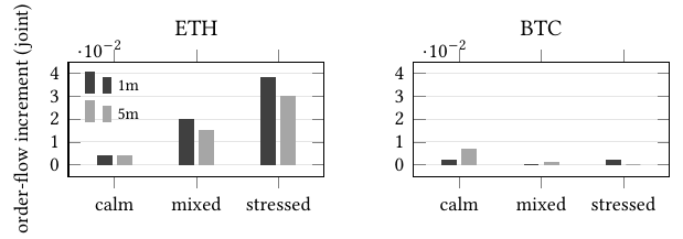
ETH's joint increment runs 0.004, 0.020, and 0.038 from calm to mixed to stressed at one minute, and 0.004, 0.015, and 0.030 at five minutes. Stressed over calm is 0.038 / 0.004 = 9.5 at one minute and 0.030 / 0.004 = 7.5 at five. All six ETH cells clear their own shuffle, with a 90 percent event-cluster interval above zero. On BTC, one cell of six clears, the five-minute calm bar, and the stressed bars are at or below their null at both horizons. No BTC regime clears at both horizons, which is why the pooled five-minute scrape does not get a BTC claim. Adding the UTC hour to the shuffle blocks leaves 0.989 of the held-out rows still permutable, and the ETH cells still clear that stricter null. A Benjamini-Hochberg correction, which caps the expected share of false calls, at q = 0.05 across the twelve symbol-horizon-regime cells, leaves every ETH cell standing and still gives BTC no two-horizon pass.

A model given trade flow and no book is worse than the book-only tree at both horizons. He does not print the size of that shortfall. Flow keeps its place as an overlay on the book.

The tree adds about as much as the state did, and both logits go negative

Look at the five-minute bar in the last group. It is the tree's gain over the coarse label. The first group is a different baseline: the coarse label's gain over the marginal frequencies. The two logit groups are also versus the coarse label, and both sit below zero.

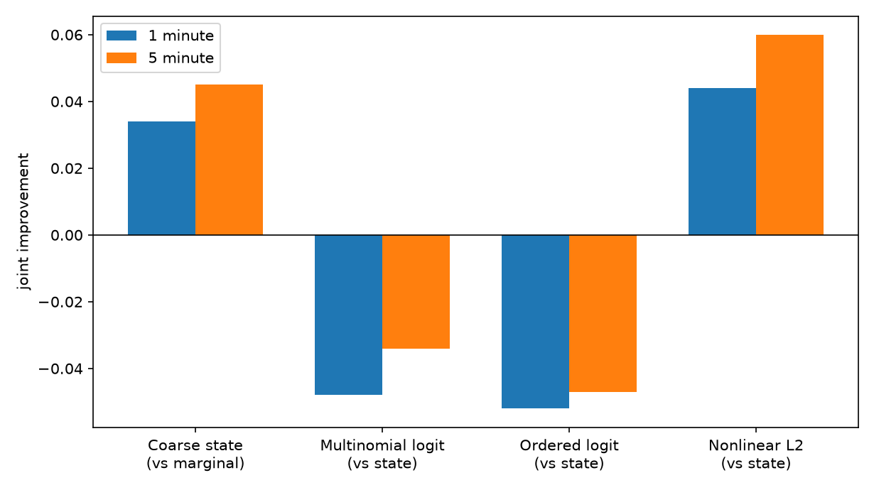
Three numbers off that chart, at two decimals: the five-minute tree is 0.06, the one-minute multinomial logit is −0.05, and the five-minute multinomial logit is −0.03. The coarse state is 0.03 at one minute and 0.045 at five, the ordered logit is −0.05 at both horizons, the tree is 0.04 at one minute and at five minutes 0.05 on BTC and 0.07 on ETH, and pooled order flow is 0.01, carried by ETH at 0.02, while BTC stays under 0.01 and is not established.

The tree is a histogram gradient-boosted classifier, depth at most three, sixty rounds, learning rate 0.05, ridge penalty 1.0. Its inputs are summaries of depth, imbalance, the best-quote spread, and mid-price changes over the pre-event window. He does not list the scales inside "multi-scale." The 90 percent bootstrap intervals on its joint gain are [0.041, 0.046] at one minute and [0.057, 0.062] at five, both clear of zero. He says both logit intervals lie entirely below zero and does not print their endpoints. The continuous book, handed to a linear model, loses to the three-bin label built from the same measurements. The extra gain shows up when the model is allowed a shallow nonlinearity, and that gain is about the size of the state's own gain over the marginal model.

Accuracy for the tree is 0.586 at one minute against a majority-class rate of 0.571, and 0.554 at five minutes against 0.532. The gaps are 0.586 − 0.571 = 0.015 and 0.554 − 0.532 = 0.022. He also says the mixed state covers about 0.55 of the rows, a coarser round number for that majority class. Calling every row mixed already lands near the base rate. The loss moved because the probabilities on the other two labels moved.

Widen from the label, and leave flow off BTC

Use the pre-event label to change a width or a size before the print, and leave the flow feature off BTCUSDT until a test clears at both horizons. A stressed book can carry a stressed-to-stressed probability as high as 0.456, against a stressed share of about 0.25, about 1.8 times that share. Widen or cut size off that probability. A direction still needs a price model, and he did not fit one.

I am against reading the tree's joint-score gain as a spread you have collected. The paper reports no fee, no markout (the price move after a fill), and no simulator. The snapshot cannot recover queue position, your own fill probability, or a sub-second impact. A one-minute top-20 picture has no queue in it. The accuracy gap above is what an argmax rule picked up. A quoting rule consumes the probabilities, which is why he scored a proper score, and those probabilities still do not name a fill.

Do not swap the label for a realized-volatility tercile and call it the same control. That tercile, cut on the training fold only, improves the marginal model by 0.008 at one minute and 0.015 at five. He says the liquidity state exceeds it by 0.026 and 0.029 on the unrounded differences, with a 90 percent event-cluster interval above zero. Subtracting the printed scores gives 0.034 − 0.008 = 0.026 and 0.045 − 0.015 = 0.030. The one-minute pair matches. The five-minute pair is 0.001 off the unrounded gap he states, which is the rounding note he already attached, not a second result. The old article "Crypto Isn't Structurally Alien: Roll/VPIN/Amihud Predict Distribution Shifts" found a spread estimator that was mostly volatility persistence under another name. He ran that objection on purpose, and the book label still beat the volatility cut.

Fit the terciles, and every other transform, on the months before the test month. A cut estimated on the whole 2023–2026 panel leaks the evaluation month into the label. He left type, region, and importance out of the fit. The result covers windows the calendar located. A model that is also told the release is CPI is a different test, and this paper does not run it.

The old article "State-Dependent (In)Efficiency: Meta-Learning a Directional-Change Threshold" picks a price-reversal size from a small menu and reports an out-of-sample Sharpe of 1.34 on crypto futures, gross of costs. That is a state used as a trading switch. This paper's state is a label of the book, and it reports no Sharpe. Leave it that way until you have fills. A reinforcement-learning execution layer, or a language-model context layer, has to beat the depth-three tree on this joint score, out of sample, under the event-cluster bootstrap, before its extra parameters count. The tree's settings are the bar: depth three, sixty rounds, learning rate 0.05, ridge 1.0. ETH versus BTC is two contracts. He calls the asymmetry a two-point observation. Code and derived artifacts wait on acceptance, and the raw books are licensed, so you cannot clone the interval from a public dump tonight.

KEY POINTS

• Cap the severe-descriptor count at two. Relative spread, negated top-20 depth, and absolute imbalance each add one when they sit in the training-fold top tercile, and a count of three is still stressed.
• Leave the release minute out of the features. Aggregate from five minutes before the print up to the print, and score the book from the print out to one minute or five minutes. Fit every cut on earlier months.
• Average the negative-log-likelihood gain and the Brier gain. The coarse label's five-minute joint improvement over the marginal model is 0.045, from printed components 0.061 and 0.028 whose average is 0.0445.
• Throw out a layer that loses to the layer under it. The multinomial logit is −0.048 at one minute against the coarse label. The depth-three tree is +0.060 at five minutes, with a bootstrap interval [0.057, 0.062].
• Add trade flow only on top of the book, and only where the shuffle loses. ETH's stressed one-minute joint increment on the full panel is 0.038, against 0.004 when the book is calm. BTC has no regime that clears at both horizons.

References

• The Signal Ceiling: Why No Single-Bar OHLCV Edge Beats Costs in MNQ
• Crypto Isn't Structurally Alien: Roll/VPIN/Amihud Predict Distribution Shifts
• State-Dependent (In)Efficiency: Meta-Learning a Directional-Change Threshold
• When Does Order Flow Matter? State-Dependent L2 Liquidity-State Transitions in Crypto Futures, Joohyoung Jeon

A note on AI. The ideas, research, analysis, and conclusions in this article are my own. I use AI tools to help with editing and wordsmithing, because English is not my first language, and I am not shy about that. AI-generated ideas and AI-assisted writing are not the same thing: the first is empty slop from a generic prompt, the second is a tool for communicating years of real research more clearly. Judge the work by its substance, not by whether software helped polish the prose.