5.51 Crypto Isn't Structurally Alien: Roll/VPIN/Amihud Predict Distribution Shifts

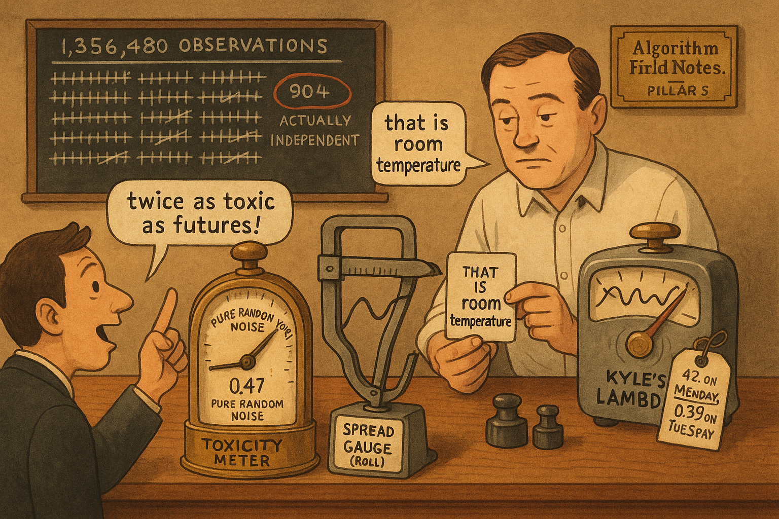
Easley, O'Hara, Yang and Zhang take five textbook microstructure measures, compute them on Binance one-minute bars for BTC, ETH, XRP, SOL and ADA over January 2021 to July 2023, and ask a random forest to call the sign of tomorrow's change in the return distribution. Two numbers carry the paper. Crypto VPIN averages 0.47 against the 0.22 that the same authors found in E-mini and crude futures, which they read as heavier toxicity. And accuracy on the sign of the change in realized volatility runs 0.56 to 0.58, well above the 0.50 a coin flip gives you. I reproduced the machinery behind both numbers and neither one means what the paper says it means. The VPIN gap is an artifact of the estimator, and the volatility accuracy leans on a feature that is mostly a volatility measure wearing a spread estimator's name. One finding survives both objections, and the abstract buries it.

The five features are the Roll measure, the Roll impact measure, Kyle's lambda, the Amihud illiquidity ratio and VPIN, each computed for each of the five coins over a trailing window W of 50 or 100 one-minute bars. Each coin's model therefore sees 25 features: its own microstructure and the other four coins'. The labels are the sign of the change, 1,500 bars ahead, in realized volatility, autocorrelation, skewness, kurtosis and the Jarque-Bera statistic. The choice of 1,500 bars, roughly a trading day, exists to stop the label at bar t and the label at bar t+1 from sharing data. Hold on to that number, because it decides how much evidence the paper has.

The Roll measure is a volatility measure with extra steps

Roll's 1984 estimator recovers an effective spread from the bid-ask bounce: with a constant spread and no drift, consecutive price changes have a negative autocovariance equal to minus the squared half-spread. The paper drops the sign and takes an absolute value.

$$ \text{Roll}_t \;=\; 2\sqrt{\bigl|\operatorname{cov}(\Delta P_t,\; \Delta P_{t-1})\bigr|}, \qquad \Delta p_t = p_t - p_{t-1} $$ $$ \text{if } \Delta p \text{ is AR(1) with volatility } \sigma \text{ and autocorrelation } \rho: \qquad \text{Roll}_t \;=\; 2\,\sigma\,\sqrt{|\rho|} $$

The first line is the paper's equation, taking the covariance between the vector of price changes over the window and the same vector lagged one bar. The second line is what that expression collapses to when price changes follow a first-order autoregression: the covariance is rho times sigma squared, so the square root pulls out sigma times the square root of the absolute autocorrelation. The absolute value is what makes it usable at all, since crypto minute bars often show positive autocovariance and the original estimator would demand a square root of a negative number. It also destroys the interpretation. A momentum-driven positive autocovariance and a bounce-driven negative one of equal size print the identical "spread".

Read the elasticities off the second line. Roll is linear in sigma and square-root in the absolute autocorrelation, so doubling volatility doubles Roll while doubling autocorrelation raises it by 41%. Worked example on a BTC window where minute price changes have a standard deviation of 2 dollars and an autocorrelation of 0.05: Roll equals 2 times 2 times the square root of 0.05, which is 0.894 dollars. Push the autocorrelation to 0.10 and Roll goes to 1.265, up 41%. Leave the autocorrelation at 0.05 and push volatility to 4 dollars instead, and Roll goes to 1.789, up 100%. The feature answers to volatility twice as hard as it answers to the autocorrelation it is supposed to be measuring.

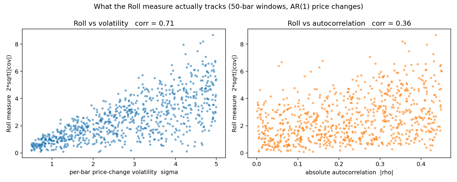
I simulated 800 windows of 50 AR(1) price changes, drawing sigma uniformly between 0.5 and 5 and rho uniformly between minus 0.45 and 0.45, then computed the paper's Roll measure on each. Correlation with sigma comes out at 0.71, correlation with the absolute autocorrelation at 0.36. Those exact levels depend on the ranges I drew from, so treat the ratio rather than the levels as the result: Roll loads on volatility about twice as hard as on autocorrelation, which is the elasticity the algebra predicted.

Now put that next to the paper's own feature-importance chart for the label it predicts best.

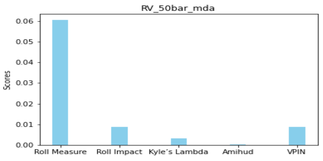
The Roll measure scores a mean decreased accuracy of 0.058 for predicting the sign of the change in realized volatility. Every other feature sits under 0.01, and Amihud registers 0.001. So the forest predicts future volatility mostly from one feature, and that feature is a scaled estimate of current volatility. Volatility clusters. The paper's strongest result is a well-behaved model rediscovering volatility persistence through a proxy, and the conclusion that the Roll measure "provides a microstructure foundation for the momentum observed in crypto prices" does not follow from an importance score on a statistic that tracks sigma first and rho second.

The old article "Bid-Ask Spread From OHLC: The GMM Estimator That Beats Roll/CS" is the relevant comparison. That work keeps the spread interpretation intact by combining several OHLC-based estimators under GMM, pushing minute-level correlation with a high-frequency benchmark from 56% to 89% and cutting non-positive estimates from 34% of observations to 0.02%. The absolute-value patch here takes the opposite route: it guarantees a positive number by throwing away the sign that made the number a spread.

VPIN's null value is 0.50, and Binance prints 0.47

VPIN splits each bar's volume into buyer-initiated and seller-initiated parts using bulk volume classification, then averages the absolute imbalance. Write out the paper's version and the volume cancels.

$$ \text{VPIN}_t=\frac{1}{W}\sum_{i=t-W+1}^{t}\frac{\bigl|V_i^{S}-V_i^{B}\bigr|}{V_i}, \qquad V_i^{B}=V_i\,Z\!\left(\frac{\Delta p_i}{\sigma_{\Delta p}}\right), \qquad V_i^{S}=V_i-V_i^{B} $$ $$ \Longrightarrow\qquad \text{VPIN}_t=\frac{1}{W}\sum_{i=t-W+1}^{t}\Bigl|\,1-2\,Z\!\left(\tfrac{\Delta p_i}{\sigma_{\Delta p}}\right)\Bigr| $$

Substitute the buy volume into the numerator and every V cancels: the buy side is V times Z, the sell side is V times one minus Z, their difference is V times the quantity two Z minus one, and dividing by V leaves the absolute value of one minus twice Z. The measure contains no volume information at all. It is an average of standardized one-minute price changes pushed through the normal CDF, which is worth knowing before anyone builds a toxicity dashboard on it.

Worked example over two bars. The first bar moves plus 0.8 standard deviations, so Z equals 0.7881 and the term is the absolute value of one minus 1.5762, which is 0.5762. The second bar moves minus 0.1 standard deviations, so Z equals 0.4602 and the term is 0.0797. The two-bar VPIN is 0.328. Now do it in general. Under a pure random walk with Gaussian price changes, Z of a standard normal draw is uniform on the unit interval, so the absolute value of one minus twice a uniform is itself uniform on the unit interval, and its expected value is exactly 0.500. Zero information, no toxicity, no informed trader anywhere: the paper's VPIN still reads 0.50.

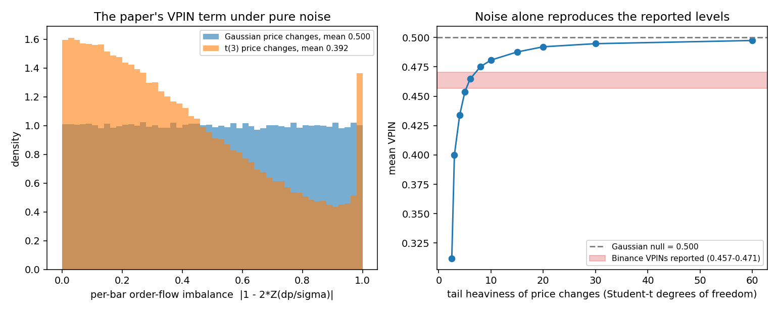
Fat tails push it down rather than up. When price changes are leptokurtic, standardizing by the window's own standard deviation packs most bars near zero and Z clusters near one half, so the imbalance term shrinks. Simulating 400,000 draws, Gaussian price changes give a mean of 0.4996 and Student-t with 3 degrees of freedom gives 0.392. The Binance VPINs in Table 1 run from 0.4566 for XRP at 100 bars to 0.4705 for ETH at 50 bars, averaging 0.4678 across the five coins at 50 bars. That band lands exactly where pure noise with a tail index around 5 to 7 degrees of freedom lands. Crypto minute returns have tails in that range.

The 0.22 for E-mini and crude comes from Easley, Lopez de Prado and O'Hara's 2012 construction, which aggregates buy and sell volume across a whole equal-volume bucket before taking the absolute difference. Summing signed imbalances first lets them cancel; taking absolute values bar by bar first, as this paper does, forbids cancellation. Jensen's inequality guarantees the bar-by-bar version prints higher, on any data, informed or not. The paper concedes "a slightly different methodology" in a single clause and then treats 0.47 against 0.22 as evidence of greater information-based trading in crypto. Two estimators with different null values are not a comparison.

The sample holds 904 observations, not 1.4 million

The paper reports no standard errors on any accuracy figure. It predicts 1,500 bars ahead and it makes a prediction every minute, so consecutive labels share 1,499 of 1,500 bars of look-ahead. Independent observations arrive once every 1,500 minutes, not once a minute.

$$ N_{\text{eff}}=\frac{T}{h}, \qquad \mathrm{SE}=\sqrt{\frac{0.25}{N_{\text{eff}}}}, \qquad z=\frac{\widehat{\mathrm{acc}}-0.5}{\mathrm{SE}} $$

T is the number of one-minute bars in the sample and h is the 1,500-bar look-ahead, so their ratio counts non-overlapping blocks. The standard error uses the binomial variance of a fair coin, one quarter, because the null being tested is accuracy of 0.50. Worked example: January 2021 through July 2023 spans 942 days, or 1,356,480 minute bars, which divided by 1,500 gives 904 independent blocks. The standard error is the square root of 0.25 over 904, or 0.0166. Realized volatility at 0.5816 sits (0.5816 minus 0.5) over 0.0166, a z of 4.91. Autocorrelation at 0.5317 gives a z of 1.91.

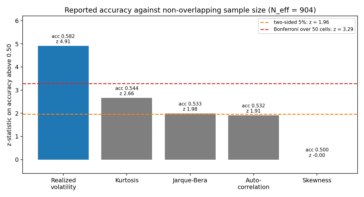
Realized volatility clears any bar you set. Kurtosis clears 5% and nothing else. Jarque-Bera and autocorrelation sit on the 1.96 line, and skewness is a coin flip by the paper's own admission. Apply the multiple-testing tax and the picture tightens: the paper runs five labels across five coins at two window lengths, which is 50 cells before you count the crypto-winter split, and a Bonferroni threshold at 5% over 50 tests sits at a z of 3.29. One label survives. That calculation is also generous, because it credits the model with the full sample when only a held-out test slice produced those accuracies, and the paper never states the split. Shrink the test set to a third and every z falls by a factor of 1.7, leaving realized volatility at 2.8 and nothing else standing.

Two more things follow from the same arithmetic. The crypto-winter robustness test compares aggregated accuracy of 0.5379 before November 2021 against 0.5395 after, and calls the 0.0016 gap "remarkable stability". The two subperiods hold 301 and 603 independent blocks, so the standard error on their difference is 0.035 and the test cannot see a true gap smaller than about 7 accuracy points. Stability that loose is compatible with the market changing a great deal. And the logistic-regression check in Figure 10 reports realized-volatility accuracy of 0.61 against the forest's 0.58. A linear model beat 100 trees on 25 features, which is what you expect when a single feature carries the signal.

Kyle's lambda and Amihud never worked here, and the definitions say why

$$ \lambda_t=\frac{p_t-p_{t-W}}{\sum_{i=t-W}^{t} b_i V_i}, \qquad b_i=\operatorname{sign}(p_i-p_{i-1}), \qquad \text{Amihud}_t=\frac{1}{W}\sum_{i=t-W+1}^{t}\frac{|r_i|}{p_i V_i} $$

Kyle's lambda divides a price change over the window by the net signed volume over the same window. Over 50 bars of two-sided flow that denominator is a near-cancelling sum, so lambda measures the reciprocal of net imbalance rather than price impact. Worked example: 500 million dollars of gross volume over the window with a 1% net imbalance gives a 5 million dollar denominator, so a 30 dollar BTC move prints a lambda of 6 times ten to the minus six. Same 30 dollar move, same gross volume, but a 0.01% net imbalance, and the denominator is 50,000 dollars and lambda prints 6 times ten to the minus four, a hundredfold jump from a quantity that has nothing to do with liquidity. The paper's own Tables 1, 9 and 10 show the damage: BTC's 50-bar lambda reads 42.22 before November 2021, 0.391 after, and 15.99 over the full sample, while the 100-bar version of the same statistic reads 1.26. A twelvefold gap between a 50-bar and a 100-bar estimate of the same quantity is not a market changing, it is an estimator failing. Kyle's lambda earns a near-zero mean decreased accuracy in every table, and that is the model correctly ignoring noise.

The Amihud definition has a separate problem. Section II defines V_t as the dollar volume in bar t, yet Amihud divides by p_i times V_i and Roll impact divides by p_t times V_t. Under the stated definition both expressions count price twice and neither is the Amihud ratio. Read V as share volume and all three formulas become the standard ones while the prose becomes wrong. I keep the printed form and flag the inconsistency rather than pick a reading for the authors, but note which way it cuts: Amihud scores near-zero importance everywhere, including a negative 0.0009 for realized volatility before crypto winter, and a mis-specified denominator is a plausible reason.

What survives

The cross-coin ranking survives all of it. Each coin's own Roll measure dominates its own predictions, and after that the Roll measures of BTC and ETH outrank every other coin's features.

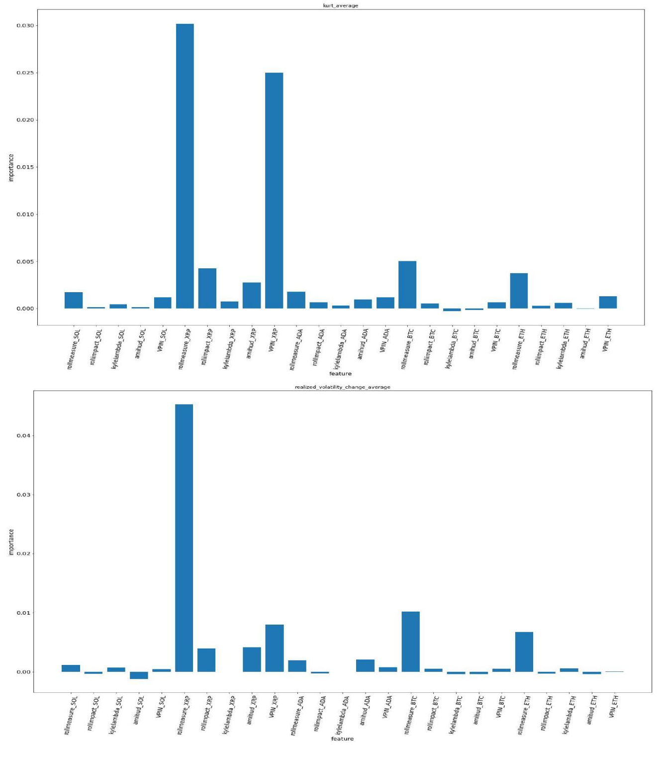
For XRP kurtosis, the own Roll measure scores 0.030, own VPIN 0.025, and then BTC's Roll measure at 0.005 and ETH's at 0.004 lift clear of everything else, while SOL and ADA features sit at zero. That pattern repeats across all five coins. Since the Roll measure is largely a volatility proxy, the honest reading is that BTC and ETH volatility leads volatility in the smaller coins at a one-day horizon, and no other pair of coins carries information. That is a real and usable statement about crypto structure, consistent with Makarov and Schoar on where crypto price discovery concentrates, and it does not depend on any of the estimators behaving as advertised. It also survives the winter split, and unlike the accuracy comparison, a rank ordering of features is a coarse enough claim that low statistical power does not sink it.

Two of the paper's own summary numbers do not reconcile with its tables, so check them before you quote them. The introduction claims an AUC above 0.55 averaged across currencies and variables, while Table 2 reports aggregated AUC of 0.5381 at 50 bars and 0.5304 at 100 bars. The introduction also gives a per-label AUC range of 0.54 to 0.61, while the tables produce 0.53 to 0.58 for the four predictable labels; the 0.54 to 0.61 range is the futures result the authors quote later from their 2021 work. I keep the tables.

The title claim holds. Crypto market dynamics are not structurally alien, and the same measures that predict distribution shifts in futures predict them on Binance at similar magnitudes. Nimalendran, Pathak, Petryk and Qiu reach a compatible verdict from variance-ratio tests rather than machine learning, so the inefficiency itself is not in dispute. Trading on it is another matter. Predicting the sign of the change in one-day-ahead realized volatility at 0.58 accuracy is a vol-forecasting result, and you can already get that from a GARCH fit on the same bars without a 25-feature forest. The paper is a careful negative for four of its five labels and a tautology-adjacent positive for the fifth.

KEY POINTS

• The Roll measure the forest leans on is not a spread estimate. Taking the absolute value of the autocovariance makes it equal 2 times sigma times the square root of the absolute autocorrelation, so it responds to volatility with elasticity 1 and to autocorrelation with elasticity 0.5. Simulated 50-bar windows give correlation 0.71 with sigma against 0.36 with the absolute autocorrelation.
• Predicting the sign of the change in realized volatility from a volatility proxy at 0.58 accuracy is volatility clustering, not a microstructure foundation for momentum. The Roll measure scores mean decreased accuracy of 0.058 while every other feature sits under 0.01.
• The paper's VPIN reduces to the average of the absolute value of one minus twice the normal CDF of standardized price changes, so volume cancels out entirely. Its expected value under a Gaussian random walk is exactly 0.500, and the reported Binance range of 0.457 to 0.471 is what noise with 5 to 7 degrees of freedom of tail weight produces.
• Comparing 0.47 to the 0.22 that Easley, Lopez de Prado and O'Hara found in futures compares two estimators with different null values. Their version aggregates signed volume across a bucket before taking absolute values; this one takes absolute values bar by bar, which Jensen's inequality guarantees prints higher on any data.
• With a 1,500-bar look-ahead over 942 days, the sample holds 904 independent observations and the standard error on accuracy is 0.0166. Realized volatility gives z of 4.91, kurtosis 2.66, Jarque-Bera 1.98, autocorrelation 1.91, skewness zero. Against a Bonferroni threshold of 3.29 for 50 label-coin-window cells, one label survives.
• The crypto-winter test compares 0.5379 to 0.5395 across subperiods holding 301 and 603 independent blocks. The standard error on that difference is 0.035, so the test cannot detect a true gap under about 7 accuracy points. Read the result as no detectable change, not as stability.
• Kyle's lambda divides by net signed volume, which nearly cancels over 50 bars, so a hundredfold change in net imbalance moves lambda a hundredfold with the same price move. BTC prints 42.22 before winter, 0.391 after, and 1.26 at a 100-bar window. Its near-zero importance scores are the forest ignoring noise.
• Take the cross-coin ranking as the durable finding: BTC and ETH Roll measures are the only cross-coin features with importance anywhere, so BTC and ETH volatility leads the smaller coins at a one-day horizon and no other pair carries information.

References

• Flow Toxicity and Liquidity in a High-frequency World - Easley, Lopez de Prado, O'Hara (Review of Financial Studies, 2012)
• Microstructure in the Machine Age - Easley, Lopez de Prado, O'Hara, Zhang (Review of Financial Studies, 2021)
• Trading and Arbitrage in Cryptocurrency Markets - Makarov, Schoar (Journal of Financial Economics, 2020)
• Informational Efficiency of Cryptocurrency Markets - Nimalendran, Pathak, Petryk, Qiu (Journal of Financial and Quantitative Analysis, 2024)
• Microstructure and Market Dynamics in Crypto Markets - Easley, O'Hara, Yang, Zhang (ssrn-4814346)