5. Microstructure Alpha August 28, 2026 10 min

5.49 The Worst-Kept Secret: Imbalance Is the MM's Optimal Response, Not Alpha

Order book imbalance predicts price moves because a market maker who knows the true price posts it that way to manage her own inventory risk, not because it leaks information.

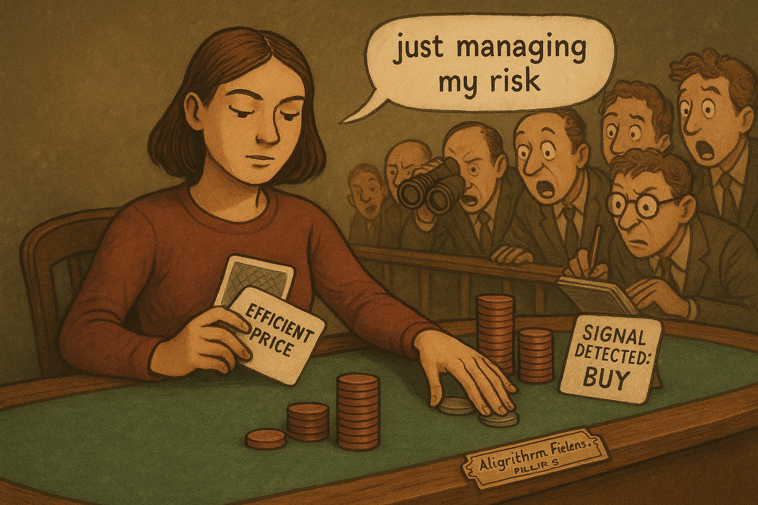
Sasha Stoikov called it the "worst-kept secret of high-frequency trading" in a 2014 seminar: the volume imbalance in a limit order book predicts the next mid-price move. Define it as I = (q^b − q^a)/(q^b + q^a), where q^b is the size resting at the best bid and q^a the size at the best ask. Push I toward 1 and the next tick tends to be up. Push it toward −1 and the next tick tends to be down. Huang, Lehalle and Rosenbaum documented it in 2015, Lehalle and Mounjid confirmed it in 2017, Sfendourakis and Muni Toke again in 2023. Every writeup since treats the correlation as a free signal: watch the depth, trade the flip.

Pulido, Rosenbaum and Sfendourakis build a model that removes the mystery entirely. Their market maker already knows where the price is going. The imbalance sitting in her book is not information leaking out of someone else's trade. It is the volume she chose to post, given what she knows, to maximize her own expected utility. Run her optimization and the predictive imbalance falls out as a byproduct, not an assumption. You are not detecting an informed trader's footprint. You are reading a solved control problem.

A market maker who already knows the answer

Strip the setup to its parts. There is an efficient price S, the "true" value nobody quotes directly, following a Bachelier random walk: dS_t = σ dW_t, plain Brownian motion with volatility σ. There is a mid-price P that sits on a tick grid and only moves in discrete half-tick jumps, governed by the model with uncertainty zones from the old article's neighboring literature (Robert and Rosenbaum, 2011): when S drifts far enough from P, P snaps to catch up. And there is a single market maker who observes S directly, which nobody trading against her does. She is the platform's only liquidity provider.

Because the stock is large-tick, the spread is stuck at one tick almost always, so she cannot move the price. Her only lever is size: how much she posts at the best bid (q^b) and the best ask (q^a). Market orders arrive against those quotes as two independent Poisson processes, and their arrival rate depends on Y := S − P, the gap between the efficient price and the tradeable one. When Y is large and positive, buy orders arrive faster because market takers see the same drift she does. She does not control that arrival rate or its size. Market orders show up whether or not she is quoting, which rules out price manipulation by construction: there is no channel through which her quotes change the tape's behavior, only how much of that behavior she captures.

$$ I = \frac{q^b - q^a}{q^b + q^a} $$

Worked example: she posts 30 units at the bid and 10 at the ask. I = (30 − 10)/(30 + 10) = 0.5. An outside observer sees a book tilted toward buying pressure and, per the empirical studies above, expects the next move to be up. In this model that expectation is correct, but not because 20 extra units of buy-side size are "information." They are her answer to a question she already knows the answer to.

An efficient price nobody else can see

The jump rule is concrete enough to check with numbers. Take the paper's own example parameters: tick size δ = 0.01, uncertainty-zone parameter η = 0.2. The mid-price jumps up by half a tick the instant S climbs to P + δ(η + 1/2). Plug in: 0.01 × (0.2 + 0.5) = 0.01 × 0.7 = 0.007. So the efficient price has to run 0.7 of a full tick past the current mid-price before the quoted price catches up. Below that, P sits still, S wanders, and the gap Y = S − P widens and narrows on its own.

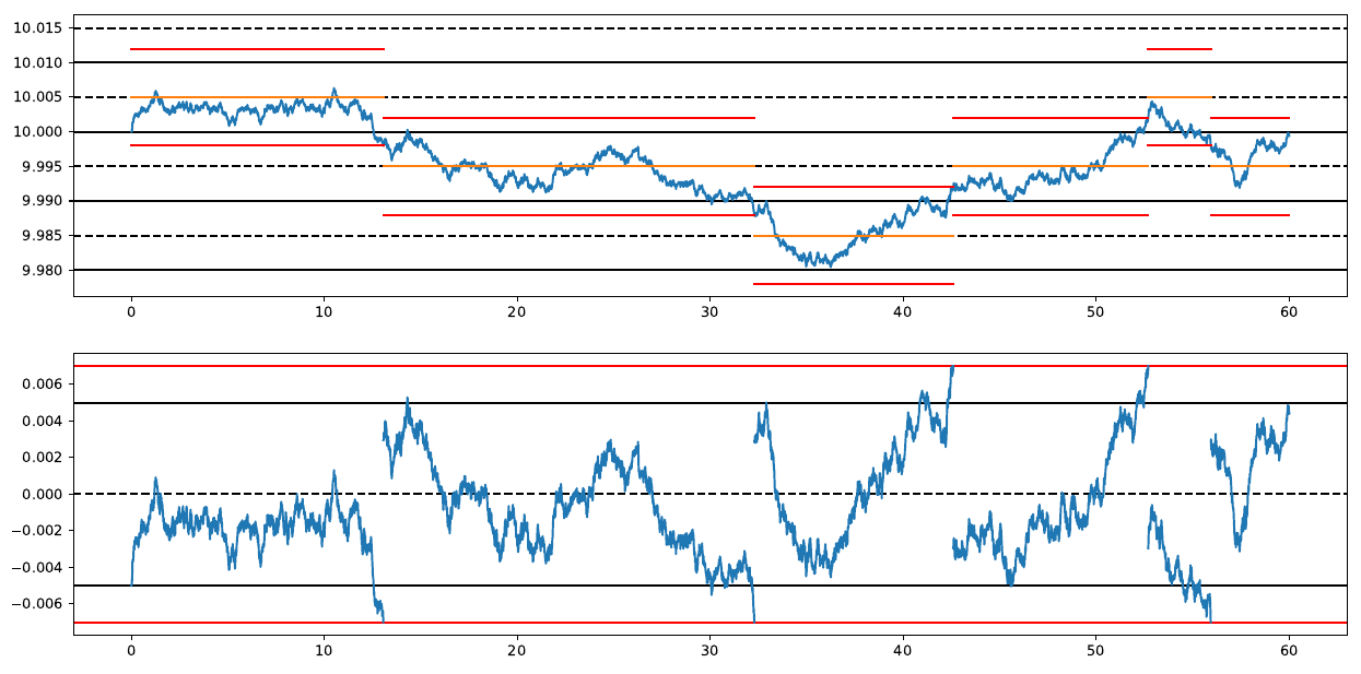
Sample path of the efficient price S (top, blue) against the sticky mid-price P (top, orange steps) with uncertainty-zone barriers in red, and the resulting gap Y = S minus P (bottom)

Read the top panel first: S wanders continuously while P only steps when S has drifted far enough away, exactly the δ(η + 1/2) = 0.007 rule above. The bottom panel is Y itself, oscillating inside a band and occasionally testing the red barrier lines, at which point P catches up and Y snaps back toward zero because S is continuous but P just jumped by half a tick. η itself is not a free parameter you have to guess: Robert and Rosenbaum show it can be estimated from tick data as η̂ = N^c/(2N^a), the count of price-move continuations over twice the count of alternations, so this whole barrier distance is checkable against real quote data, not fitted to make the chart look nice.

What one fill is worth

The market maker's actual decision reduces to comparing two numbers every instant: what she nets if a sell order hits her bid, versus what she nets if a buy order lifts her ask. From the model's profit-and-loss decomposition, filling one unit on the ask side pays δ/2 − Y, and filling one unit on the bid side pays δ/2 + Y.

$$ \text{Ask fill edge} = \frac{\delta}{2} - Y, \qquad \text{Bid fill edge} = \frac{\delta}{2} + Y $$

Worked example, continuing with δ = 0.01 so δ/2 = 0.005: say Y = 0.002, meaning the efficient price sits 0.2 of a tick above the mid. Selling one unit at the ask nets 0.005 − 0.002 = 0.003. Buying one unit at the bid nets 0.005 + 0.002 = 0.007. Buying is more than twice as attractive as selling at this instant, because selling now hands away a unit at a price that is about to look cheap once S catches up, while buying locks in a discount. That asymmetry is the entire mechanism. She responds by posting less on the ask and more on the bid, which mechanically raises I. Nobody told her the imbalance formula; it falls out of comparing two fill payoffs.

Risk aversion caps the response, cleverness doesn't

If fill edges were the only consideration, she would post unlimited size on whichever side pays more and let inventory run wherever it wants. She doesn't, because she maximizes the exponential utility of her terminal profit with a risk-aversion coefficient γ, not the expected profit itself. Holding a large inventory Q exposes her to the swings of σ dW_t on every unit she carries, and exponential utility punishes that variance directly. The Hamilton-Jacobi-Bellman equation that comes out of her optimization (equation 2 in the paper) carries a running term (σ²γ²Q²)/2 that acts as a continuous inventory penalty, independent of any single trade's edge.

$$ \text{Inventory risk penalty rate} = \frac{\sigma^2 \gamma^2 Q^2}{2} $$

Worked example: take σ = 0.005 and Q = 15 units, the same values used in the paper's own sensitivity charts. At γ = 0.5, the penalty rate is (0.005² × 0.5² × 15²)/2 = (0.000025 × 0.25 × 225)/2 ≈ 0.0007, about a fourteenth of a tick. Quadruple the risk aversion to γ = 2 and the rate jumps to (0.000025 × 4 × 225)/2 ≈ 0.01125, more than a full tick. Because the penalty scales with γ squared while a trade's edge only scales linearly with γ through the exponential's argument, doubling risk aversion doesn't double the caution, it roughly quadruples it. That is why the paper's own numerical experiments show a more risk-averse market maker pulling her quoted volumes back toward zero inventory well before her physical limit, and why the imbalance she posts depends on Q as well as on Y: a market maker sitting on inventory of −15 needs a much smaller Y before she's willing to buy aggressively than one sitting on +15.

The dial: quoted imbalance as a readout of S minus P

Solve the full control problem numerically and plot the resulting imbalance against Y for a few fixed inventory levels, and you get a monotone staircase from −1 to 1.

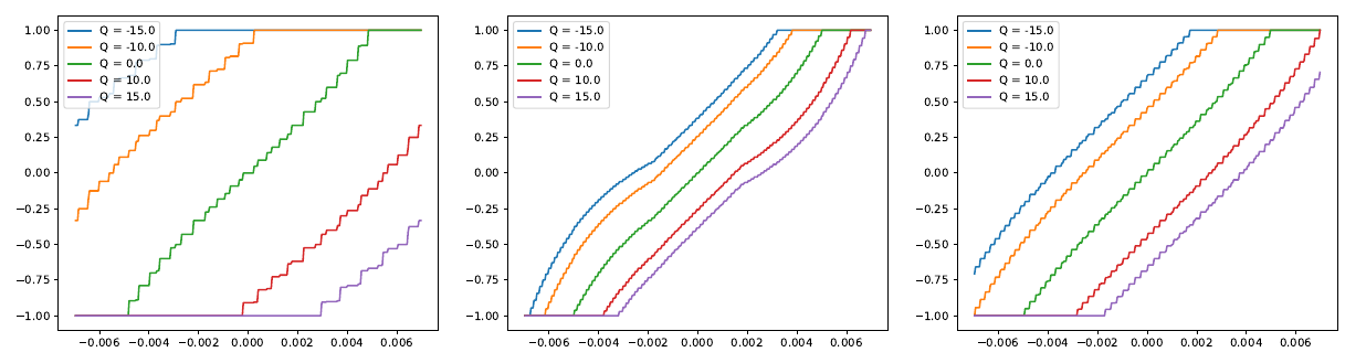
Optimal quoted imbalance as a function of Y = S minus P, for inventory levels Q from -15 to +15, across three parameter configurations

Each panel fixes a different combination of risk aversion, volatility and order-flow intensity; within a panel, each line is one inventory level. Read the leftmost panel at Y = 0, meaning the efficient price sits exactly on the mid: the Q = −15 line (she is short 15 units and needs to buy back) is already pinned near an imbalance of +1, quoting almost nothing on the ask and heavily on the bid. The Q = +15 line (she is long 15 and needs to sell) is still pinned near −1 at that same Y = 0 and only starts climbing once Y has moved a noticeable distance toward positive territory. Being long and being short shift the entire staircase sideways along the Y axis; a long inventory needs a stronger bullish signal before she'll flip to aggressive buying, exactly as the risk-penalty math above predicts.

One inconsistency worth flagging rather than quietly fixing: the paper's introduction defines volume imbalance as I = (q^b − q^a)/(q^b + q^a), the standard convention this article uses throughout, and states correctly that a higher I predicts a higher next-period price. But the paragraph introducing Figure 4 in Section 5.1 defines the plotted quantity as (q^a − q^b)/(q^a + q^b), the opposite sign. Since the same paragraph and Figure 3 both establish that q^a is decreasing and q^b is increasing in Y, that reversed formula would produce a curve falling from 1 to −1 as Y rises, not the rising staircase the paper plots and describes. The chart and the surrounding prose only make sense under the introduction's original sign convention; the formula printed in Section 5.1 looks like a transcription slip in the source, and this article keeps the source's plotted result (imbalance rising with Y) rather than silently rewriting the paper's formula for it.

A free byproduct: sizing the tick

Because the model already computes how often market orders hit each side, it also answers a question regulators and exchanges care about: what tick size maximizes traded volume? Too small a tick and each fill barely pays the market maker anything, so she trades less; too large a tick and her posted price sits too far from the efficient price for market orders to bother crossing it. Running the platform's expected-volume objective across a grid of tick sizes at σ = 0.005 (using the empirical relation η = η₀√(δ₀/δ) from Dayri and Rosenbaum, with η₀ = 0.2 and δ₀ = 0.1 as anchors), the paper finds an optimum at δ = 0.0032. Push volatility higher and the optimal tick grows with it: at σ = 0.0075 it is 0.0044, at σ = 0.01 it is 0.0064, and at σ = 0.015 it is 0.015. A more volatile stock needs a fatter tick so the market maker earns enough per fill to keep quoting through the extra risk. This is one derived application, not the paper's main claim, but it shows the same coupled HJB system pays for itself twice: once to explain imbalance, once to size the venue.

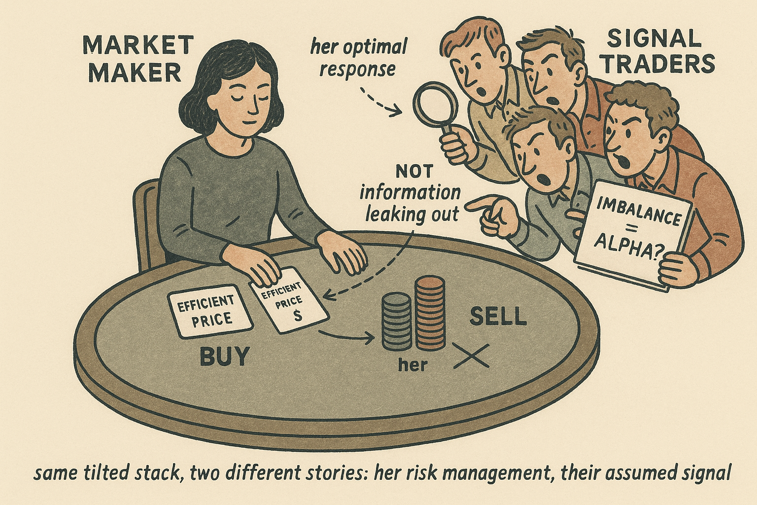
Treat all of this as a caution against any strategy built on "buy when imbalance spikes." The old article "Order Book Imbalance: The First Microstructure Feature to Test" tested the correlation empirically and found it real; this model explains why the correlation exists without needing any informed trader on the other side of the book at all. A rational, uninformed-about-your-order market maker generates a predictive imbalance purely as a side effect of managing her own inventory risk against a price she can see and you cannot. A retail signal built on it captures a mechanical echo of someone else's risk aversion, not leaked information. The three-pillar quoting framework from the old article "The Three Pillars of Market Making: Fair Price, Spread, Skew" already treats skew as an inventory-management tool; this paper is the formal proof that the same skew, observed from outside, is indistinguishable from a forecasting signal.

KEY POINTS

Volume imbalance I = (q^b − q^a)/(q^b + q^a) is treated across the microstructure literature as a predictive signal; this model shows it is instead the optimal quoting response of a market maker who already observes the efficient price and cannot be gamed by market orders she does not control.
The efficient price S follows a Bachelier walk (dS = σ dW) while the mid-price P only jumps by half a tick once S drifts δ(η + 1/2) away from it; with δ = 0.01 and η = 0.2, that barrier is 0.007, checkable against real data since η itself is estimable as N^c/(2N^a).
Each fill has a clean payoff: δ/2 − Y on the ask side, δ/2 + Y on the bid side. When Y > 0, buying pays more than selling, so the market maker posts more bid size than ask size, mechanically raising I.
Risk aversion, not signal cleverness, caps her inventory: the HJB equation's penalty term (σ²γ²Q²)/2 grows with the square of γ, so quadrupling risk aversion multiplies the inventory cost sixteenfold and pulls her book back toward zero well before her hard limit.
Solved numerically, the optimal imbalance is a monotone staircase from −1 to 1 in Y = S − P, shifted sideways by current inventory; a short position needs less bullish evidence to trigger aggressive buying than a long position does.
The paper's own Section 5.1 prints the plotted imbalance formula with a flipped sign relative to its introduction and relative to what the chart actually shows; this article keeps the plotted result and flags the formula as likely mistranscribed rather than silently correcting it.
As a free byproduct, the same coupled HJB system picks an optimal tick size: 0.0032 at σ = 0.005, rising to 0.015 at σ = 0.015, since a more volatile stock needs a fatter tick to keep the market maker's per-fill edge worth the risk.

References

- High-Frequency Trading in a Limit Order Book - Avellaneda and Stoikov (2008)
- A New Approach for the Dynamics of Ultra-High-Frequency Data: The Model with Uncertainty Zones - Robert and Rosenbaum (2011)
- The Micro-Price: A High-Frequency Estimator of Future Prices - Stoikov (2018)
- Simulating and Analyzing Order Book Data: The Queue-Reactive Model - Huang, Lehalle and Rosenbaum (2015)
- On Bid and Ask Side-Specific Tick Sizes - Baldacci, Bergault, Derchu and Rosenbaum (2023)
- Understanding the Worst-Kept Secret of High-Frequency Trading - Pulido, Rosenbaum and Sfendourakis (2024)