4. Market Structure Notes August 25, 2026 11 min

4.74 FX Edge Lives in Other Markets (cross-asset series)

FX edge sits in the graph: EM stocks lead by a month, G10 loops pay daily, and FX futures Sharpe jumps from 0.16 to 0.66 once other asset classes are wired in.

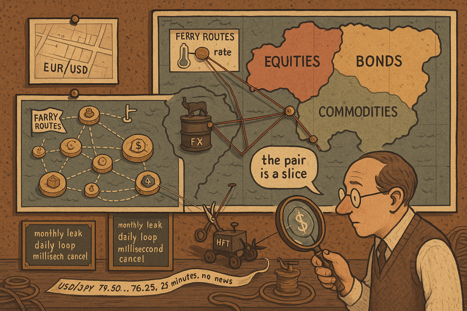
A currency futures book built from other currency futures scores a Sharpe of 0.16. The same contracts, wired into a graph that also contains equities, bonds, and commodities, jump the FX sleeve to 0.66. That is Pu, Roberts, Dong, and Zohren, 64 futures, 2000 to 2022, volatility-targeted to 15%. Phylaktis and Yamani ran the pairwise version of the same instinct and got a harsher split: a country's own stocks and bonds forecast next month's exchange rate in emerging markets, 0.59% a month net of costs, and fail the random-walk test in the G10. Hong and Klabjan then showed that even those G10 pairs still pay once they are treated as a ten-currency graph with interest rates on the nodes. The old article "Network Momentum as a Cross-Asset Factor" already made the graph the unit of analysis. This piece is that claim run on FX, at three clocks, with the plumbing that can cut the wires.

The pair is a slice. The object is the graph of stocks, bonds, rates, and other currencies.

Pairwise first: stocks lead FX, and only where the market is slow

Phylaktis and Yamani, covered in the old article "Stocks and Bonds Predict FX — But Only in Emerging Markets," put one differential in front of one currency. Local stock return minus US stock return, one month, 28 countries, November 1989 to December 2019. The forecast is a regression.

$$ \Delta s_{i,t+1} = \alpha + \beta \left( r^{E}_{i,t} - r^{E,US}_{t} \right) + \varepsilon_{i,t+1} $$

Delta-s is next month's log change in foreign-currency units per one US dollar, so a negative number means the foreign currency strengthened. The term in parentheses is the equity differential. Beta is the whole signal. The bond model swaps in government-bond returns; the combined model uses both. Across the combined model the equity coefficient came in negative for every basket: minus 0.105 developed, minus 0.129 emerging, minus 0.083 global. Negative means a hot local equity market, relative to the US, is followed by a stronger local currency next month. That is return-chasing: foreign capital buys the equity, and has to buy the currency to do it.

Work the emerging coefficient. Stocks beat the US by 2 percentage points this month. Predicted delta-s is minus 0.129 times 2, which is minus 0.258%, call it a quarter percent of appreciation, so the rule buys the currency. One coefficient, one differential, one month.

The bar is the random walk, unbeaten in developed FX since Meese and Rogoff. They score it with out-of-sample R-squared.

$$ R^{2}_{OOS} = 1 - \frac{MSFE^{\chi}}{MSFE^{RW}} $$

MSFE is mean squared forecast error. The ratio of the model's squared misses to the random walk's, subtracted from one. Positive means the model beat the coin flip. The emerging combined model posts a relative MSFE of 0.95, so R-squared is 0.05: squared errors about 5% below the random walk. (The table caption says "percent units"; Rel-MSFE of 0.95 only matches if 0.05 is a fraction, so the caption and the arithmetic disagree, and the arithmetic is the one that is internally consistent.) The developed combined model posts 1.016, R-squared minus 0.016, worse than doing nothing.

Clark-West t-stats, the formal nested-model test, draw the line. Emerging equity 3.113, emerging combined 2.724, both past 1%. Developed equity 0.626, developed combined 1.405, neither clearing 10%. Bonds fail the full sample in both groups. Trading the sign of the forecast, net of half the bid-ask, earned 0.30% a month on emerging equity signals and 0.59% a month combined, about 7% a year, with positive skew, beating carry and currency momentum. Developed currencies produced nothing tradable.

The pairwise channel is real, and it is a leak. Emerging markets are thinner, more segmented, slower to absorb the equity flow. Developed markets arbitrage the same flow before a monthly signal can cash it. That is the old article's result, and it is also the trap: stop there and G10 FX looks like a dead letter.

One hop wider: other currencies and the rate on the node

Hong and Klabjan, in the old article "Graph Learning for FX: Interest-Rate-Parity Statarb Done Right," refuse the pair. Ten currencies are nodes. Tradable exchanges are edges. Government-bond interest rates sit on the nodes. The exchange rate rides the edge. A graph neural network passes messages along that web, which is the structure interest-rate parity already implies.

Covered parity is the lock.

$$ (1 + Y^{f}_{i})\, F_{ij} = (1 + Y^{f}_{j})\, X_{ji} $$

The left side grows a unit at country i's risk-free rate and converts forward. The right side converts spot into j and grows at j's rate. If the two sides disagree, borrow the cheap leg and lend the rich one. Work it: i pays 5%, j pays 1%, spot from j to i is 1.00. The forward from i to j has to be 1.01 over 1.05, about 0.962, so the high-rate currency trades at a forward discount. Uncovered parity swaps the forward for the expected future spot. Either way the rate on the node carries information about the edge, which is why a flat table of pairs is the wrong input.

The residual they hunt is the loop that should close and does not.

$$ \text{Loop payoff} = X_{ik}\, X_{kj}\, X_{ji} - 1 $$

Convert one unit of i into k, k into j, j back into i, subtract the starting unit. Product above one is a paying loop. USD to EUR at 0.92, EUR to JPY at 162.0, JPY back to USD at 0.0068: 0.92 times 162.0 is 149.04, times 0.0068 is 1.0135. The product lands at 1.0135 dollars, a 1.35% sliver. Aiba and coauthors documented those slivers as a real interaction among FX rates. Fenn and coauthors called the spot version a mirage once the time between the screen and the fill is in the model. Hong and Klabjan take Fenn's objection as the problem statement: decide at t minus 1, execute at t where the fill is random, hold overnight, convert home at t plus 1, and maximize expected gain over the standard deviation of that gain, not raw profit.

Against a linear-program benchmark that uses the same rate forecasts, the graph method lifts information ratio 61.89% and Sortino 45.51%, cuts annual volatility 52.23% and max drawdown 44.77%, and pays for it with 22.73% less raw return: 4.80% a year versus 6.19% on a USD base, vol 0.68% versus 1.41%. Divide 4.80 by 0.68 and the ratio is about 7.1, against 6.19 over 1.41, about 4.4. The table prints "Info. Ratio" as 43.86 versus 27.21, labeled in percent; those figures match a daily ratio times 100 (4.80% over 252 days, 0.68% annual vol, daily IR near 0.44), not the annual Sharpe. The 61.89% lift is the same ratio either way.

Chaboud, Hjalmarsson, Vega, and Chiquoine already showed that algorithmic traders on EBS eat triangular opportunities at a five-second clock and cut the absolute autocorrelation of five-second returns, because machines reprice faster than people. That is not a contradiction. The five-second triangle is gone. The daily, rate-informed, lag-aware residual across ten currencies is a different object. G10 pairs fail Phylaktis's monthly stock regression and still contain a graph residual Hong can trade, on paper, with no transaction costs in the backtest and unlimited borrowing assumed. Treat the 4.80% as a method result, not a paycheck.

Widen again: the FX node in a 64-asset graph

Pu and coauthors, in the old article "Network Momentum as a Cross-Asset Factor," take the next hop. Sixty-four futures across commodities, equities, fixed income, and FX. No firm-level tie connects cotton to the dollar. They learn the graph from prices: eight momentum features per contract (volatility-scaled returns at 1 day, 1 month, 3 months, 6 months, 1 year, plus three MACDs), then a convex program that puts large edges between assets whose feature vectors look alike and zeros the rest.

Network momentum for a target is the edge-weighted average of its neighbors' features. The target's own past return does not enter.

$$ \tilde{u}_{i,t} = \sum_{j \in \mathcal{N}(i)} \tilde{A}_{ij,t}\, u_{j,t}, \qquad y_{i,t} = \tilde{u}_{i,t}^{\top} \beta + b $$

The first sum is the propagated feature vector. The second is one cross-sectional OLS across all assets, predicting next day's volatility-scaled return; the sign is the trade. Work a scalar version. Neighbors weighted 0.5, 0.3, 0.2, with one-month vol-scaled momentum of plus 1.2, minus 0.5, and plus 0.8. Propagated signal: 0.5 times 1.2 plus 0.3 times minus 0.5 plus 0.2 times 0.8, which is 0.60 minus 0.15 plus 0.16, so plus 0.61. Long the target, even if its own recent return was flat.

The ablation is the FX result that belongs in this article. Rebuild the network inside FX alone, then trade the same FX contracts off the full cross-class graph.

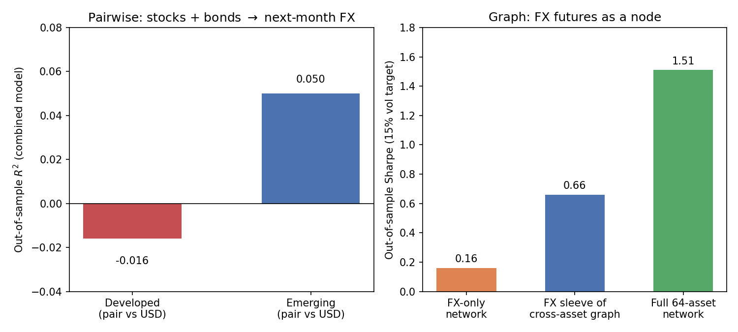
Two-panel figure: left, Phylaktis combined-model out-of-sample R-squared, negative for developed pairs versus USD and plus 0.05 for emerging; right, Pu et al. Sharpe as the graph around FX widens, from 0.16 FX-only to 0.66 as an FX sleeve of the cross-asset graph to 1.51 for the full 64-asset book

FX-only network: Sharpe 0.16, 2.4% a year at the 15% vol target, 40% of days underwater. The same FX sleeve off the full graph: Sharpe 0.66, 9.7% a year, underwater time down to 29%. Equities make the same jump, 0.30 to 0.95. The information that prices a currency future is sitting in the bonds, commodities, and equity indexes that share its momentum regime. Intra-class edges still carry more weight than inter-class edges alone (Sharpe 1.21 versus 0.91 for the full book), and the two are only 0.51 correlated, which is why the full graph beats either piece. Inter-class links are the ingredient that makes FX more than FX. They are not the whole meal.

Gross, daily rebalance. The 64-asset book stays positive up to about 3 basis points of pseudo-cost and goes negative at 5. Nobody should read 1.51 as a number that survives a futures roll and a real commission.

The graph has a kill switch

Golub, Dupuis, and Olsen, in the old article "HFT Supplies Liquidity Until It Doesn't: FX Flash-Crash Cascades," put the microstructure under the three papers above. The FX market is a mesh, not a ladder: EBS and Reuters at the center, Currenex and Hotspot as ECNs, Oanda as an FCM, CME futures off to the side, about 1.4 trillion dollars of spot a day. On EUR/USD, Ultra-HFT posts 61.6% of orders and fills 6.8% of them. Manual traders post 3.7% and fill about half. The depth on the screen is 93% cancellable.

Chaboud's machines, the same cohort that closes five-second triangles, do not trade with each other as much as random matching would predict. Their strategies are more correlated than humans'. On average that is useful: prices update faster, arb dies, five-second autocorrelation falls. The same commonality means that when the shared signal says exit, they exit together and act as one enormous trader. Cespa and Foucault write the fragility: a small liquidity drop in one asset feeds back into a market-wide crash, with a bad equilibrium that looks like May 6, 2010.

March 17, 2011 is the clean FX case. USD/JPY around 79.50 at 05:55 Tokyo, below 76.50 twenty-five minutes later, 300 pips, no fresh fundamental in that window. Retail stop-losses into a thin tape, banks yank quotes or widen until their bids sit under the last print, more stops, down to 76.25. Recover to 78.23, then another automated stop-out wave, about two billion dollars, down to 77.10. HFT and traditional makers had both left. Designated market makers widened so far the obligation was theater.

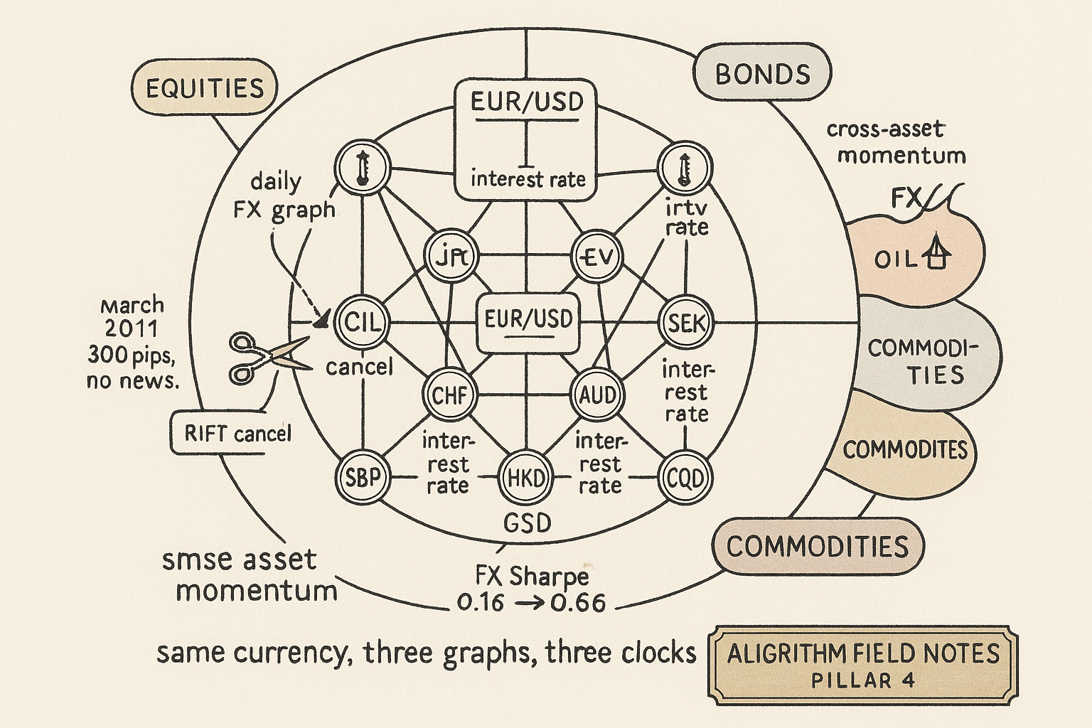
So the graph the other three papers trade is not a fixed object. At a monthly clock, emerging equity flow still leaks into the currency. At a daily clock, G10 loops and cross-asset momentum still show up in closes. At a millisecond clock the edges are quotes, and quotes vanish in a cascade. A strategy that sizes off yesterday's graph and hits a market order into a 05:55 Tokyo tape is trading a different graph than the one it estimated.

Hau and Rey, and Kremens and Martin, give the economics that makes the slower clocks possible: equity and currency returns are correlated through capital flow, and a stock-based currency risk premium has genuine predictive content. Phylaktis is that premium as a monthly trading rule. Hong is the intra-FX, intra-rate version of the same interrelatedness. Pu is the extra-FX version, learned from prices because cotton has no quanto on the dollar. Golub is the reminder that all of it clears through a book whose majority-posted liquidity is optional.

Three clocks, one object

Put the four papers on one desk and the disagreement dissolves into horizon.

Monthly, pairwise, 28 countries: stocks (and, after 2013, bonds) predict emerging FX and lose to the random walk in the G10. The edge is a flow lag, and it has an off switch. From September 2006 to April 2013, through the crisis dollar spike, the combined strategies made no reliable money and the emerging bond rule lost 0.68% a month. From May 2013 to December 2019 the same bond rule made 0.47% a month. One six-year window carries the full-sample 0.59%.

Daily, ten currencies plus government-bond rates: G10 pairs that failed the monthly stock test still contain a graph residual. Information ratio up 61.89% versus an LP that ignores the lag, return down 22.73%, no costs in the test, drawdowns in 2020, 2022, and 2024 when regimes the training set never saw arrived.

Daily, 64 futures: FX as a class is a weak momentum book on its own (Sharpe 0.16) and a decent one once equities, bonds, and commodities are allowed to speak (0.66). The full cross-asset network prints 1.51 gross and dies somewhere between 3 and 5 basis points.

Millisecond: the transmission lines are HFT quotes. They tighten spreads and kill triangles in calm, and they drop the quote in a cascade. Retail is on the wrong side of both.

A desk that stares at EUR/USD, or even at a basket of G10 pairs, is using the unit of analysis Phylaktis already falsified for developed markets and Pu already beat by a factor of four on FX futures. The trade is: estimate the graph that is live at your clock, trade the node off its neighbors, and assume the edges can go to zero without a press release.

KEY POINTS

The unit of analysis for FX is the graph of stocks, bonds, rates, and other currencies. A pair versus the dollar is a slice of that graph, and the slice is where the edge is weakest.
Pairwise, Phylaktis and Yamani: local minus US stock (and bond) returns forecast next month's FX in emerging markets, Clark-West t of 3.11 equity and 2.72 combined, 0.30% and 0.59% a month net of costs. Developed currencies fail the random walk. The leak is slow, segmented, and off from 2006 to 2013.
Intra-FX, Hong and Klabjan: currencies as nodes, rates as node features, loops as the residual. Against an LP that assumes a fill at the observed rate, information ratio up 61.89%, vol down 52%, return 4.80% versus 6.19%. Five-second triangles are already gone (Chaboud); this is a daily, lag-aware residual, costless in the paper, not a paycheck.
Cross-asset, Pu et al.: FX-only network Sharpe 0.16; the same FX sleeve off a 64-asset graph 0.66; full book 1.51 gross, 22% a year, 2000 to 2022. The extra alpha is in the links between classes. Daily turnover kills it past about 3 basis points.
Microstructure, Golub, Dupuis, Olsen: Ultra-HFT posts 61.6% of EUR/USD orders and fills 6.8%. Correlated machines close arb in calm and withdraw together in stress. March 2011 USD/JPY dropped 300 pips in 25 minutes with no news. The estimated graph is not the graph a market order hits in a cascade.
Three clocks, one object. Monthly flow (emerging equities), daily graph residual (G10 plus rates, plus cross-asset momentum), millisecond quotes. Size the node off its live neighbors, and do not assume the edges stay posted.

References

- Empirical exchange rate models of the seventies: Do they fit out of sample? (Meese and Rogoff, 1983)
- Approximately normal tests for equal predictive accuracy in nested models (Clark and West, 2007)
- Exchange Rates, Equity Prices, and Capital Flows (Hau and Rey, 2006)
- The Quanto Theory of Exchange Rates (Kremens and Martin, 2019)
- Triangular arbitrage as an interaction among foreign exchange rates (Aiba et al., 2002)
- The mirage of triangular arbitrage in the spot foreign exchange market (Fenn et al., 2009)
- Rise of the Machines: Algorithmic Trading in the Foreign Exchange Market (Chaboud et al., 2014)
- Illiquidity Contagion and Liquidity Crashes (Cespa and Foucault, 2014)
- Foreign currency forecasting in emerging markets: What can stock and bond markets tell us? (Phylaktis and Yamani, 2025)
- Graph Learning for Foreign Exchange Rate Prediction and Statistical Arbitrage (Hong and Klabjan, 2025)
- High-Frequency Trading in FX Markets (Golub, Dupuis, and Olsen)
- Network Momentum across Asset Classes (Pu, Roberts, Dong, and Zohren, 2023)