10. Cross-Sectional & Factor Investing July 9, 2026 10 min

10.15 Network Momentum as a Cross-Asset Factor

Trade an asset off the momentum of everything it's linked to, not its own. A learned cross-asset graph delivers a 1.51 Sharpe, and the alpha lives in the links between asset classes.

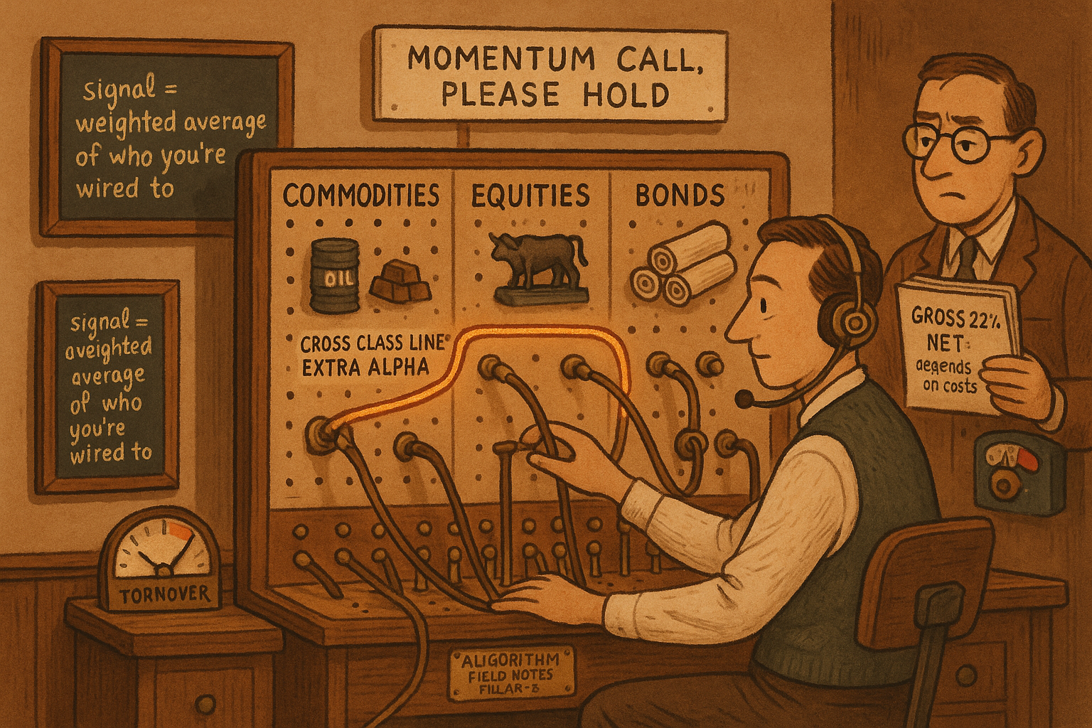
Momentum is the one factor nobody argues about. Winners keep winning, losers keep losing, and the effect shows up in stocks, bonds, commodities, and currencies across a century of data. The old article "From Intermarket Analysis to Network Momentum" pushed a harder claim: an asset's momentum can leak into the assets it is linked to, so the return of one contract carries information about the next one's future. That was the thesis. Pu, Roberts, Dong, and Zohren built the machine that tests it on 64 futures across four asset classes, and the payoff is a strategy with a Sharpe of 1.51 and 22% a year, out of sample, from 2000 to 2022, using nothing but prices.

The trick the paper solves is the one that stopped everyone before it. Momentum spillover was documented between a company's stock and its bond, or between firms in the same supply chain, because those pairs share an obvious economic tie. Cotton and the ten-year Treasury share nothing you can write down. So instead of hand-coding links, the authors learn the graph straight from the momentum data, then propagate each asset's signal along the learned edges. This is the cross-sectional, multi-asset version of the lead-lag idea the old article "Lead-Lag Relationships in Global Markets" introduced, with the graph itself as the unit of analysis instead of a single pair.

Step one: eight momentum features per asset

Before any network exists, each asset needs a momentum description. The paper uses eight features per contract per day: volatility-scaled returns over 1 day, 1 month, 3 months, 6 months, and 1 year, plus three normalized MACD indicators tuned to short, medium, and long time scales. Volatility-scaling matters because it puts a quiet bond and a wild commodity on the same axis. You divide each return by the asset's own recent volatility, so a signal of "+1" means the same size of move everywhere.

$$ \text{feature}_{i,t}(\Delta) = \frac{r_{i,\,t-\Delta:t}}{\sigma_{i,t}\sqrt{\Delta}}, \qquad \Delta \in \{1, 21, 63, 126, 252\}\ \text{days} $$

Read it as the return of asset i over the last delta days, divided by that asset's daily volatility times the square root of the horizon. Sigma is an exponentially weighted moving standard deviation with a 60-day span, so recent days count more. Say crude oil returned 8% over the past month (21 days) and its daily volatility is 2%. The denominator is 0.02 times the square root of 21, about 0.0917, so the feature is 0.08 over 0.0917, roughly 0.87. A gold contract that also returned 8% but at 1% daily vol scores about 1.74, twice as strong, because the same move is more impressive in a calmer asset. Stack the eight features for every asset and you have the raw material the network is built from.

Step two: learn the graph from the features

The links are learned, not assumed. Each day, the model stacks the feature matrix over a lookback window and solves a convex optimization for the adjacency matrix A, the table of edge weights that says how strongly every pair of assets is connected.

$$ \min_{A_t}\ \operatorname{tr}\!\left(V_t^\top (D_t - A_t)\, V_t\right)\; -\; \alpha\,\mathbf{1}^\top \log(A_t \mathbf{1})\; +\; \beta\,\lVert A_t \rVert_F^2 $$ $$ \text{s.t.}\quad A_{ij,t} = A_{ji,t},\quad A_{ij,t} \ge 0,\quad A_{ii,t} = 0 $$

The first term, the trace, is the Laplacian quadratic form. It equals a weighted sum over pairs of the edge weight times the squared distance between the two assets' feature vectors. Minimizing it puts big edges between assets whose momentum features look alike and near-zero edges between assets that do not. The middle log term forces every node to keep at least some connection, so nothing gets stranded. The last term, the squared Frobenius norm scaled by beta, penalizes huge weights and keeps the graph smooth. The constraints make the matrix symmetric, non-negative, and free of self-loops.

Work the intuition on two assets. If contract i and contract j have almost identical eight-feature vectors, the squared distance between them is tiny, so the optimizer pays almost nothing to set a large edge weight A between them, and it does. If their feature vectors point in different directions, the distance is large, and any weight there gets multiplied by a big number, so the optimizer drives that edge to zero. Two knobs, alpha and beta, tune how sparse the result is, picked by grid search on in-sample data. Smaller values give a sparser graph, which means each asset hears from only a few others and less noise propagates. The authors then average five graphs from lookback windows of one to five years to steady the weights, and the resulting network is stable: the Jaccard overlap of edges from one day to the next stays above 0.99 outside crises.

Step three: propagate, then regress

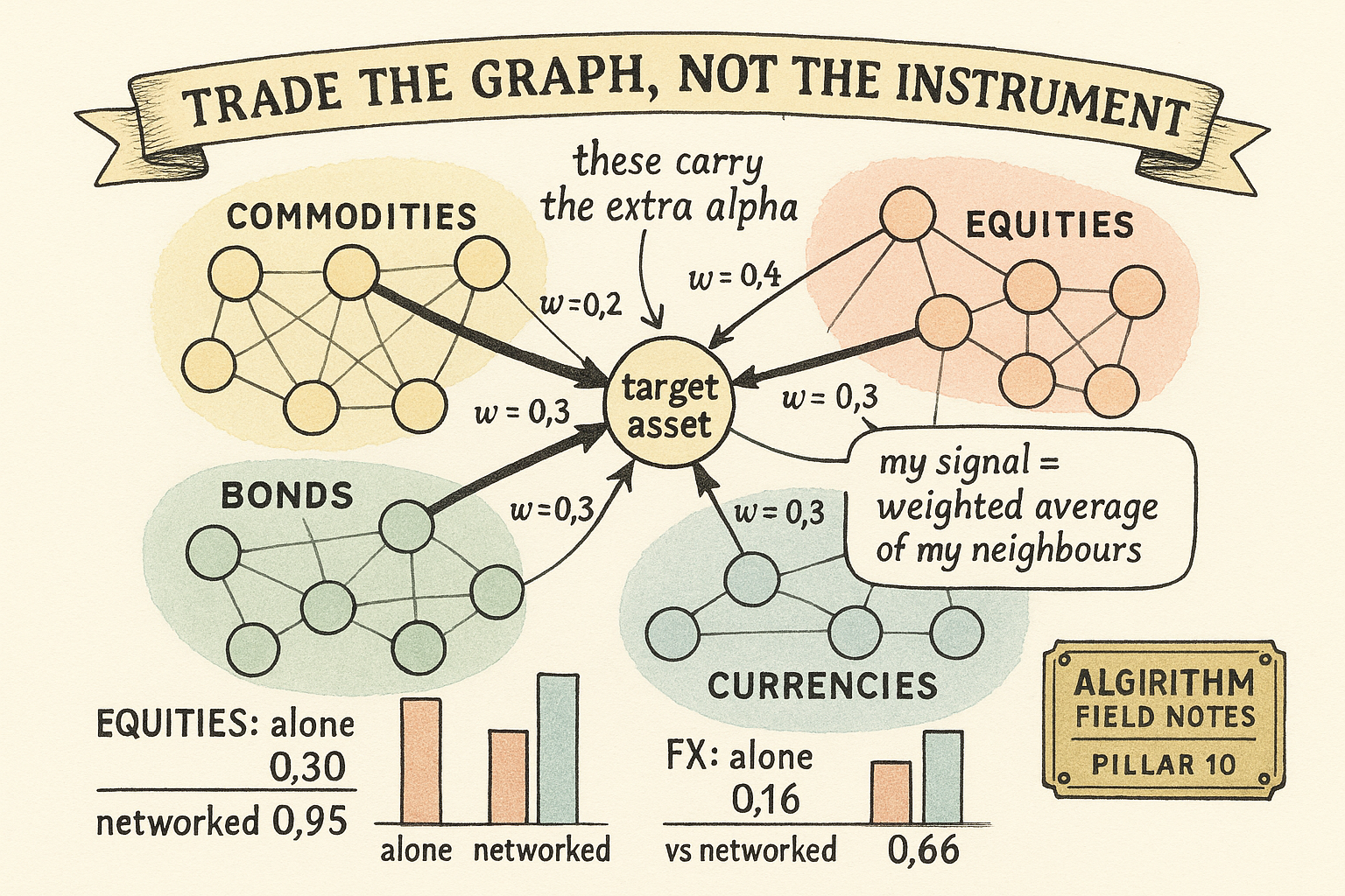
With the graph in hand, network momentum for a target asset is the edge-weighted average of its neighbors' momentum features. You do not use the asset's own past returns at all; you borrow the momentum of everything it connects to.

$$ \tilde{u}_{i,t} = \sum_{j \,\in\, \mathcal{N}(i)} \tilde{A}_{ij,t}\, u_{j,t}, \qquad\qquad y_{i,t} = \tilde{u}_{i,t}^\top \beta + b $$

The first equation says the network momentum feature vector for asset i is the sum over its neighbors j of the normalized edge weight times neighbor j's own feature vector. The second feeds that propagated vector into one cross-sectional OLS regression, trained across all assets at once, to predict the next day's volatility-scaled return. Its sign becomes the trade: positive means go long, negative means go short.

Take a scalar version. Suppose a target contract connects to three assets with normalized weights 0.5, 0.3, and 0.2, and their one-month volatility-scaled momentum reads +1.2, −0.5, and +0.8. The propagated signal is 0.5 times 1.2, plus 0.3 times −0.5, plus 0.2 times 0.8, which is 0.60 minus 0.15 plus 0.16, so +0.61. Positive, so you go long the target, even if the target's own recent return was flat or negative. That is the whole point: the position comes from the neighborhood, not the asset. The regression across eight features per neighbor is what lets the model weigh a 1-day signal against a 1-year signal and net them into one call.

The book is then volatility-targeted. Each position is sized inversely to the asset's own volatility so every name contributes the same risk, and the portfolio is scaled to a 15% annual volatility target.

$$ r^{\text{port}}_{t:t+1} = \frac{1}{N_t}\sum_{i=1}^{N_t} \operatorname{sign}(y_{i,t})\,\frac{\sigma_{\text{tgt}}}{\sigma_{i,t}}\, r_{i,t:t+1}, \qquad \sigma_{\text{tgt}} = 0.15 $$

The sign of the prediction sets direction, the ratio of target volatility to the asset's volatility sets size, and you average over all assets. A contract running at 30% annualized volatility gets a scale of 0.15 over 0.30, so half a unit; one at 10% gets 1.5 units. Same risk budget per name, which is standard trend-following hygiene.

The result: network momentum is its own signal

Run the whole thing out of sample from 2000 to 2022, retraining every five years, and the network momentum portfolio (the paper calls it GMOM) clears every benchmark. Volatility-scaled to the same 15% target, a long-only book scores a Sharpe of 0.73, a plain MACD rule 0.70, and individual momentum run through the identical regression (LinReg) 1.13. Network momentum hits 1.51, at 22% annual return, with the smallest drawdown and the shortest time underwater of the group.

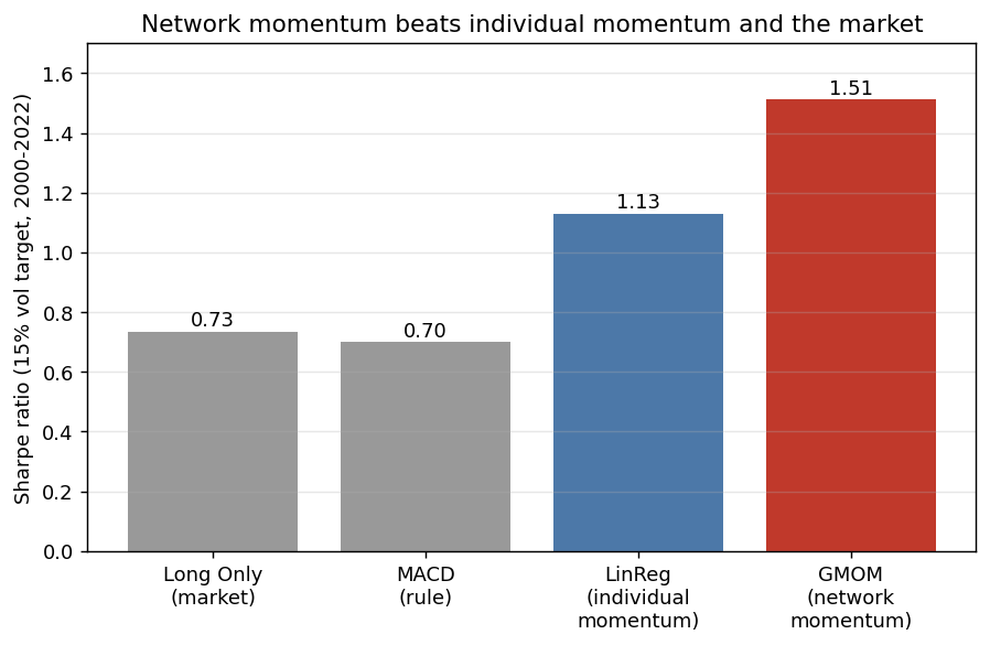
Sharpe ratios of long-only, MACD, individual momentum, and network momentum at a 15% volatility target

The comparison that matters is network momentum against individual momentum, because they eat the exact same eight features. The only difference is that network momentum propagates them across the graph first. Their return correlation is about 0.65 and they agree on direction 72% of the time, so network momentum is not a repackaging of the individual signal; it captures something the plain version misses. Averaging the two positions does not beat network momentum alone, which tells you the network version already contains most of what the individual version knows, plus extra.

Stay honest about what "1.51" includes. These are gross returns before costs, and the strategy rebalances daily, so turnover is high. The paper runs the cost sensitivity: network momentum stays positive up to a pseudo-cost of 3 basis points per trade and holds a Sharpe above 0.5 up to 2 basis points, but at 5 basis points it turns negative (−0.67), though it still beats individual momentum, which craters to −1.05 at the same cost. The edge is real in the data and more cost-robust than the individual version, but it lives or dies on execution, and nobody should read 1.51 as a number you keep.

Where the alpha actually comes from: the links between classes

The finding that earns this a place in the factor pillar is not the headline Sharpe. It is where the return comes from. The authors run the ablation you would demand: rebuild network momentum inside each asset class alone (a single-class graph), then compare it to the same class traded off the full cross-class graph. Cross-class links win in every class.

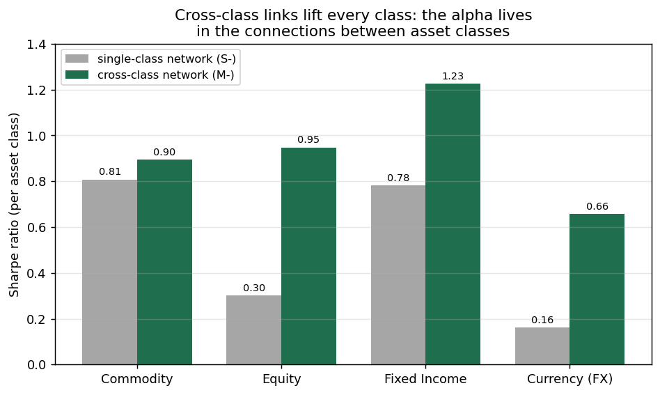
Sharpe by asset class from a single-class network versus a cross-class network

Equities are the clean tell. Built from an equity-only network, the momentum signal scores a Sharpe of 0.30. Built from the full cross-class network, the same equity trades score 0.95, more than triple. Currencies go from 0.16 to 0.66, fixed income from 0.78 to 1.23, commodities from 0.81 to 0.90. The information that helps you trade equities is not sitting in other equities; it is sitting in the bonds, commodities, and currencies that share a momentum regime with them. That is the empirical case for treating the cross-asset graph, not the single instrument, as the thing you analyze, which is exactly the graph-as-unit argument the Pillar 8 chapters on networks make.

One caution the authors surface themselves. Splitting the graph into intra-class edges only versus inter-class edges only, the intra-class version (Sharpe 1.21) beats the inter-class version (0.91), so connections within a class still carry the most weight, and the pure inter-class book took a hard hit in the 2007 to 2008 crisis. The two are only about 0.51 correlated, which is why combining them into the full graph beats either piece. Inter-class links are the ingredient that makes it better than single-class momentum; they are not the whole meal.

Reversals show up, and the regression catches them

Individual momentum has a well-known short-horizon reversal: last month's winners tend to give some back next month. Whether that reversal survives in network momentum was an open question, and the single-feature strategies could not answer it because they only carried one horizon. Feeding eight horizons into a regression lets the coefficients speak. The past 1-day return loads positive and significant in both individual and network momentum, so very recent moves continue. The past 1-month return loads negative, the classic reversal, in both. In the network version, the 3-month and 1-year signals also turn negative after 2010, which the plain individual momentum does not show, so the reversal structure of network momentum differs from the individual kind. The regression is not just a predictor here; it is a diagnostic that tells you which horizons trend and which snap back, and it lets the model net them instead of betting blindly on continuation.

What to keep and what to distrust

Network momentum is a genuine second signal, not a relabeled trend follower, and the mechanism has an economic story: momentum regimes spill across asset classes even when no company-level tie connects the instruments. The graph-learning approach is interpretable and needs only prices, which is rare for something this good on paper. The cross-class ablation is the part worth stealing even if you never trade the full system, because it says your equity book should be listening to bonds and commodities, and it measures how much that listening is worth.

The distrust is the usual short-horizon distrust. Daily rebalancing, gross Sharpe, and a cost cliff past 3 basis points mean the live version depends entirely on cheap execution and turnover control, which the authors flag and leave to future work. The training is a five-year rolling refit with a grid search over the sparsity knobs, so some of the elegance hides ordinary hyperparameter tuning. And 22 years out of sample spans only a handful of real regimes, so the 1.51 is one draw, not a law. Reproduce the number the way this pillar always tells you to: rebuild the cross-class-versus-single-class gap net of your own costs, because that gap, not the headline Sharpe, is the actual claim.

KEY POINTS

Network momentum trades an asset off the momentum of the assets it is linked to, not its own past returns. Winners' neighbors tend to win next.
The links are learned from prices, not assumed. A convex graph-learning objective connects assets whose eight momentum features (vol-scaled returns at five horizons plus three MACDs) look alike, and zeros out the rest.
A target's signal is the edge-weighted average of its neighbors' features, fed through one cross-sectional OLS regression whose sign sets the long or short position, then volatility-targeted to 15%.
Out of sample 2000 to 2022, the network momentum book (GMOM) posts a Sharpe of 1.51 and 22% a year, beating individual momentum (1.13), a MACD rule (0.70), and long-only (0.73), with the smallest drawdown.
It is a distinct signal: about 0.65 correlated with individual momentum and agreeing on direction only 72% of the time, so it adds information rather than repackaging it.
The alpha lives in the cross-class links. Trading each class off the full cross-asset graph beats trading it off a single-class graph in every class: equities jump from a Sharpe of 0.30 to 0.95, currencies from 0.16 to 0.66.
Intra-class edges still carry the most weight (Sharpe 1.21 versus 0.91 for inter-class alone), but the two are only 0.51 correlated, so the full graph beats either piece.
The regression exposes reversals: 1-day returns continue, 1-month returns reverse, and in the network version longer horizons turn negative after 2010, differing from individual momentum.
These are gross returns with daily turnover. The strategy stays positive only up to about 3 basis points of cost and goes negative at 5. Reproduce the cross-class gap net of your own costs before trusting it.

References

- Value and Momentum Everywhere (Asness, Moskowitz, and Pedersen, 2013)
- Stock and Bond Market Interaction: Does Momentum Spill Over? (Gebhardt, Hvidkjaer, and Swaminathan, 2005)
- Economic Links and Predictable Returns (Cohen and Frazzini, 2008)
- Shared Analyst Coverage: Unifying Momentum Spillover Effects (Ali and Hirshleifer, 2020)
- How to Learn a Graph from Smooth Signals (Kalofolias, 2016)
- Learning Laplacian Matrix in Smooth Graph Signal Representations (Dong, Thanou, Frossard, and Vandergheynst, 2016)
- Enhancing Time Series Momentum Strategies Using Deep Neural Networks (Lim, Zohren, and Roberts, 2019)
- Understanding Momentum and Reversal (Kelly, Moskowitz, and Pruitt, 2021)
- Network Momentum across Asset Classes (Pu, Roberts, Dong, and Zohren, 2023)
A note on AI. The ideas, research, analysis, and conclusions in this article are my own. I use AI tools to help with editing and wordsmithing, because English is not my first language, and I am not shy about that. AI-generated ideas and AI-assisted writing are not the same thing: the first is empty slop from a generic prompt, the second is a tool for communicating years of real research more clearly. Judge the work by its substance, not by whether software helped polish the prose.