10.14 Price-Path Convexity: A New Cross-Sectional Anomaly
Two stocks end the month flat, one by recovering, one by fading. The shape between the endpoints predicts next month: low-convexity stocks beat high-convexity by 0.84%/mo, and no factor explains it.
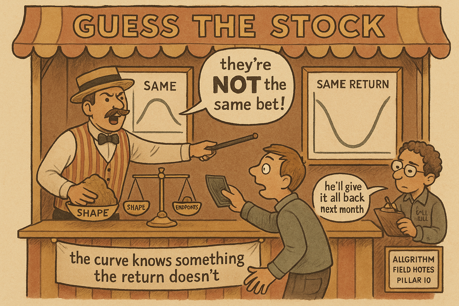
Take two stocks that both end the month flat. The first bled lower for two weeks, then clawed all the way back. The second ran up for two weeks, then gave it all back. Same start, same finish, same zero return. Sort every stock in the market by past return and these two land in the identical bucket, because return only sees the endpoints. Gulen and Woeppel show that the shape between the endpoints predicts next month, and it predicts it hard: the stock that ended by rising underperforms the stock that ended by falling by about 0.84% a month, and no standard factor touches the spread.
The old article "Wave Velocity and Acceleration: Reading When the Market Runs Out of Gas" argued that the second derivative of a price path carries an early read the level and slope miss. This is the cross-sectional version of that claim, tested on sixty years of the entire U.S. market instead of one instrument's sine fit. Return is the first derivative. Convexity, the curvature of the path, is a scaled cousin of the second derivative, and it prices the cross-section on its own.
What convexity measures, and how to compute it
Convexity compares two summaries of the same price path. Take the midpoint of the first and last closing price of the month. Subtract the average of every daily close in the month. Divide by the midpoint to standardize across price levels. That difference is the whole variable.
$$ \text{Convexity}_{it} = \frac{\dfrac{P_{1t} + P_{N_{it}}}{2} - \dfrac{1}{N_{it}}\sum_{k=1}^{N_{it}} P_{kt}}{\dfrac{P_{1t} + P_{N_{it}}}{2}} $$
Read it as midpoint of the endpoints, minus mean of the closes, over the midpoint. P-one is the first close of the month, P-N is the last close, and the middle sum is the average of all the closes in between. When the average of the closes sits below the midpoint of the endpoints, the path sagged in the middle and recovered, so convexity is positive and the path is convex, a valley. When the average sits above the midpoint, the path bulged up in the middle and faded, so convexity is negative and the path is concave, a hump.
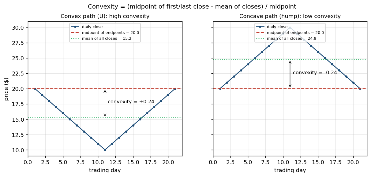
Work the paper's own example, in dollars. A stock opens the month at 20, drops 1 a day for ten days down to 10, then climbs 1 a day for ten days back to 20. First close and last close are both near 20, so the midpoint is 20. The average of all the closes is dragged down toward 15 by the trough. Midpoint minus mean is about 4.8, and 4.8 over 20 is roughly 0.24. That is a strongly convex path. Now steepen the front half: drop 1.50 a day for ten days to 5, then climb 1 a day, ending at 15. The average sinks further, the midpoint falls to 17.5, and convexity rises to about 0.42. A return measure would call both paths the same, since it only reads start and end. Convexity separates them because it weighs the whole trajectory.
The authors build it from price changes in dollars, not percentage returns, on purpose. Investors think about a stock in dollar terms as much as in percent terms (Shue and Townsend document the non-proportional thinking), and dollar changes track the path's actual dynamics better than a return that collapses to its endpoints.