10. Cross-Sectional & Factor Investing July 9, 2026 9 min

10.10 Behavioral Factors: Prospect-Theory Value and Capital-Gains Overhang

Prospect theory turns broken psychology into two factors: a TK score of how attractive a stock looks and capital-gains overhang. The prettiest stocks pay least, and the spread runs 1.24% a month.

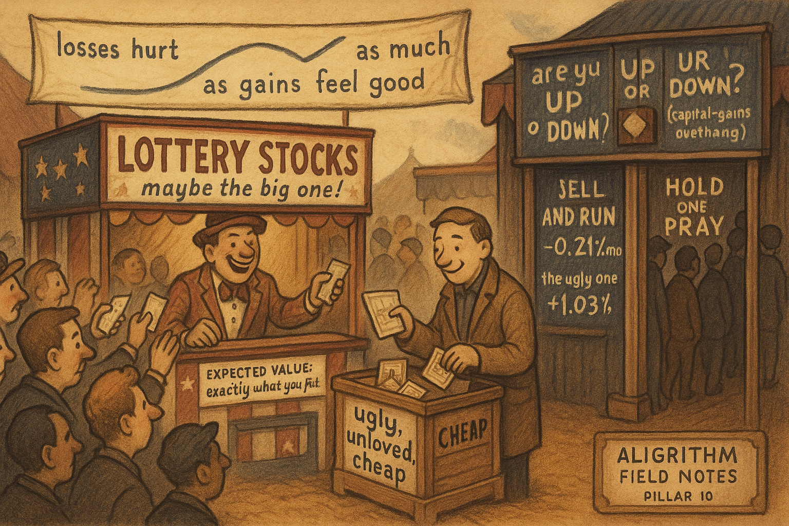
Most factor stories start with risk. You earn a premium because you hold something painful, and the pain is compensated. Behavioral factors flip the logic. Here the premium exists because other people are making a predictable mistake, and the mistake is old, robust, and written into how humans weigh gains against losses. Kahneman and Tversky mapped that machinery half a century ago, and it turns out you can turn their psychology into two tradable numbers: a score for how attractive a stock looks to a loss-averse gambler, and a score for whether the average holder is sitting on a gain or a loss.

The punchline is uncomfortable for anyone who thinks appeal and return go together. Rank stocks by how good they look through the lens of prospect theory, and the most attractive decile earns a four-factor alpha of minus 0.21% a month while the least attractive earns plus 1.03%. Long the ugly, short the pretty, and the spread is 1.24% a month with a t-statistic of 6.83. The market pays you to hold what behavioral investors cannot stomach.

The old article "The Flawed Human Brain in Trading" catalogued these biases as things to purge from your own decisions. This article does the other half: once you accept the brain is broken in known ways, you can price the breakage. It also connects to the old article "When an Alpha Metric Is U-Shaped," because the behavioral effects here are conditional, they flip sign depending on whether holders are winning or losing, and a naive linear read misses them entirely.

The value function: losses hurt more, and both ends flatten

Prospect theory replaces the textbook idea that people maximize final wealth. Instead they react to changes from a reference point, and the reaction is asymmetric. The cumulative-prospect-theory value function writes it down in closed form.

$$ v(x) = \begin{cases} x^{c} & \text{if } x \geq 0, \\ -\kappa\,(-x)^{c} & \text{if } x < 0. \end{cases} $$

Here x is the outcome measured against the reference point, a gain if positive and a loss if negative. The exponent c, between 0 and 1, bends both arms of the curve so that the tenth extra dollar matters less than the first, which is diminishing sensitivity. The coefficient kappa, bigger than 1, is loss aversion, and it steepens the loss arm so a loss stings more than the equal gain pleases. Tversky and Kahneman's estimates put c around 0.88 and kappa around 2.25.

Work a symmetric bet. A 10% gain scores 10 to the power 0.88, which is about 7.6 units of value. A 10% loss scores minus 2.25 times that same 7.6, which is minus 17.1. The loss registers 2.25 times as hard as the identical gain. Put a coin flip between plus 10% and minus 10% through this and its perceived value is minus 4.8, deeply negative, even though its expected payoff is zero. That single asymmetry is why people refuse fair gambles and, later, why they cannot sell losers.

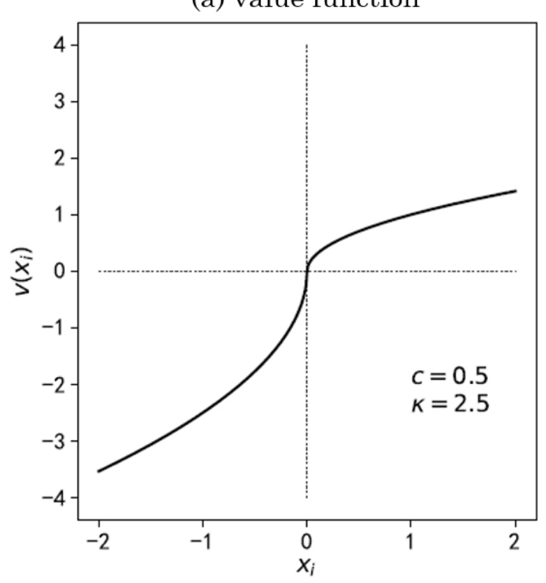
Prospect-theory value function, concave over gains and convex and steeper over losses, with c equal to 0.5 and kappa equal to 2.5

The curve makes the shape concrete. Above the reference point it is concave, so people are risk-averse in gains and grab a sure profit. Below it the curve is convex and much steeper near zero, so people turn risk-seeking in losses, holding a bad position and hoping to get back to even. That is the disposition effect in one picture, and it is the same instinct the old article "Why Traders Take Profits Too Early and Losses Too Late" warned you about from the inside.

The weighting function: rare events get overweighted

The second engine is that people do not use raw probabilities. They run probabilities through a weighting function that overweights the unlikely and underweights the near-certain.

$$ w^{-}(p) = \frac{p^{\delta}}{\left(p^{\delta} + (1-p)^{\delta}\right)^{1/\delta}} $$

The gain-side twin w-plus uses an exponent gamma instead of delta, but the form is identical. p is the true probability of an outcome, and w of p is the decision weight it actually gets. When delta is below 1, the function is an inverse-S: it lifts small probabilities above the 45-degree line and pushes large ones below. Tversky and Kahneman estimated gamma at 0.61 and delta at 0.69.

Run a 1% tail through it with delta at 0.69. The numerator, 0.01 to the power 0.69, is about 0.037. The denominator works out near 0.68, so the decision weight is roughly 0.054. A one-in-a-hundred event gets treated like a one-in-twenty event, overweighted more than fivefold. That is the whole economics of lottery tickets and cheap out-of-the-money options: people pay for the fat right tail they imagine is fatter than it is.

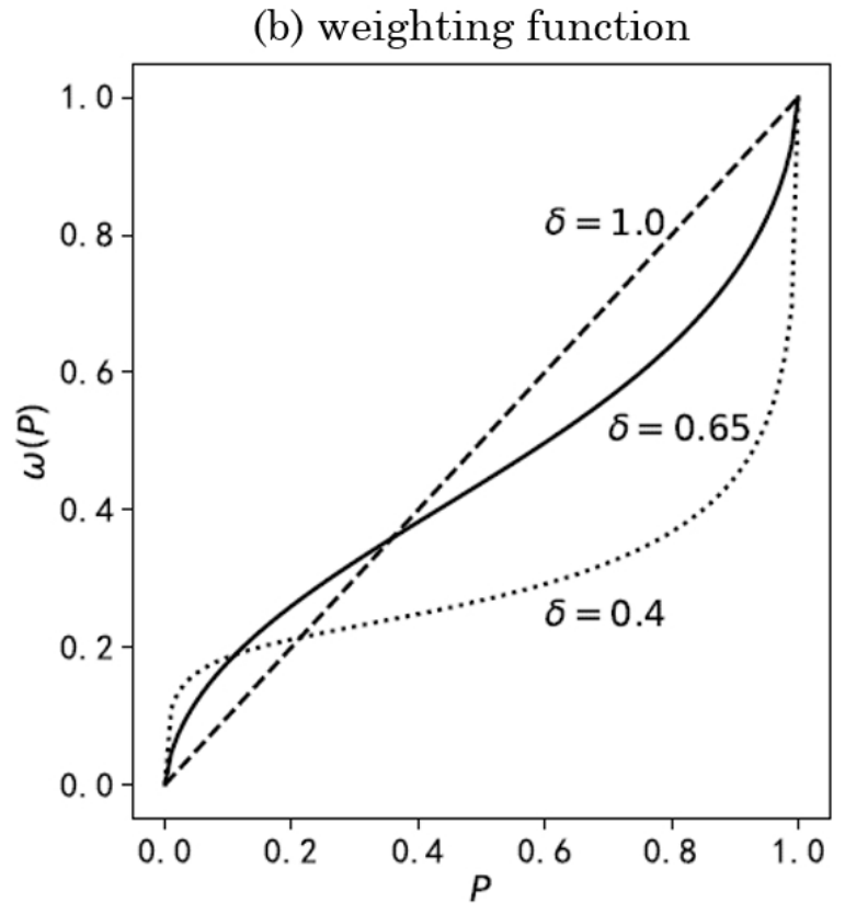
Probability weighting function for three values of delta, showing the inverse-S that overweights small probabilities and underweights large ones

The chart shows the effect getting stronger as delta falls. In markets this is why right-skewed "lottery stocks" and hot IPOs command high prices and then deliver low returns. Demand for the imagined jackpot bids the price up, and the future return pays for it.

Assembling the TK score of a stock

Barberis, Mukherjee and Wang turned these two functions into a single number per stock. You cannot know a stock's future return distribution, so they use its past 60 monthly returns as the outcome set, each with probability one over 60, and score that distribution the way a prospect-theory agent would.

$$ \text{TK} = \sum_{i=-m}^{-1} v(r_i)\left[w^{-}\!\left(\tfrac{i+m+1}{60}\right) - w^{-}\!\left(\tfrac{i+m}{60}\right)\right] + \sum_{i=1}^{n} v(r_i)\left[w^{+}\!\left(\tfrac{n-i+1}{60}\right) - w^{+}\!\left(\tfrac{n-i}{60}\right)\right] $$

Read it as a weighted average of felt value. Sort the 60 returns, run each through the value function v to get how it feels, and weight it by the decision weight from w, computed cumulatively so the extreme months in each tail get the overweighting the theory demands. The left sum handles losses with w-minus, the right sum handles gains with w-plus. A stock with a big right tail and mild losses scores high, it looks like a great prospect. Barberis and coauthors deliberately fixed the parameters at Tversky and Kahneman's originals, c 0.88, kappa 2.25, gamma 0.61, delta 0.69, so there is no fitting, no knobs to snoop.

Because attractive stocks get overbought, TK should predict returns negatively, and it does, monotonically.

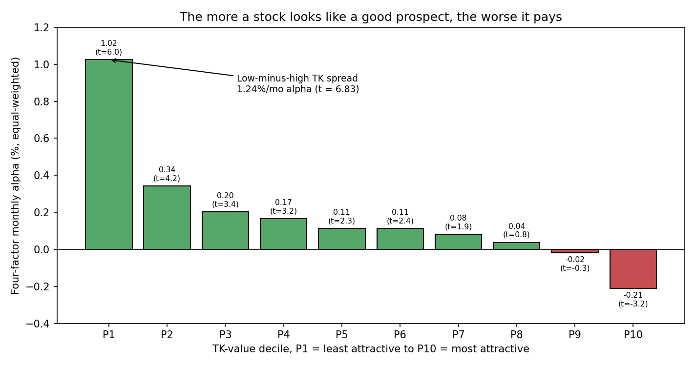
Bar chart of four-factor alpha across TK-value deciles, declining from plus 1.03% for the lowest to minus 0.21% for the highest

The lowest-TK decile earns a four-factor equal-weighted alpha of 1.03% a month at a t of 6.05, and the alpha falls almost straight across the deciles to minus 0.21% at a t of minus 3.19 for the highest. The long-short spread is 1.24% a month with a t of 6.83, and it survives a five-factor model at 1.30%. Value-weighted the spread shrinks to 0.62% but stays significant at a t of 3.67, which tells you the effect is not purely a microcap artifact. When Barberis and coauthors switched the components off one at a time, the probability weighting piece did most of the work, the overweighted tails matter more than loss aversion for the cross-section.

Capital-gains overhang: are the holders winning or losing

The value function has a second market consequence through the disposition effect. Investors sitting on gains rush to sell and lock in the win, which pushes those stocks down and leaves them undervalued, so they earn higher future returns. Investors sitting on losses refuse to sell, propping the price up and leaving the stock overvalued, so it earns lower future returns. To trade it you need to know the crowd's average cost, and Grinblatt and Han built the proxy.

$$ RP_t = \frac{1}{k}\sum_{n=1}^{T}\left(V_{t-n}\prod_{\tau=1}^{n-1}(1 - V_{t-n+\tau})\right)P_{t-n}, \qquad CGO_t = \frac{P_t - RP_t}{P_t} $$

The reference price RP is a weighted average of past prices, where each past price P at lag n is weighted by the chance that shares bought then have not turned over since, using the turnover ratio V, with k a normalizer that makes the weights sum to one. High recent turnover means old prices are unlikely to still be held, so they get little weight. Capital-gains overhang is then just the percentage distance of today's price above that average cost.

Put numbers on it. A stock trades at 50, the turnover-weighted reference price is 40, so CGO is 50 minus 40 over 50, which is 0.20. The average holder is up 20%, deep in the concave, sell-and-lock-in region of the value function, so disposition selling should press the price and set up higher future returns. A stock at 30 against a reference of 40 has a CGO of minus 0.25, holders underwater and clinging, price propped, lower future returns ahead.

The overhang is not just a standalone signal, it conditions other anomalies, and this is where the U-shape shows up. Sort by risk and by CGO together, and the low-risk anomaly reverses sign across the overhang. Among stocks whose holders are deep in losses, high-idiosyncratic-volatility names underperform low-vol names by 1.92% a month, the familiar low-risk anomaly in force. Among stocks whose holders are sitting on gains, the relationship flips positive. The difference-in-difference is 2.24% a month at a t of 7.97. The risk-return line is not flat or downward everywhere, it bends one way or the other depending on whether the marginal holder is chasing a recovery or protecting a profit. Read risk on its own and you average two opposite regimes into mush.

Where this connects

Behavioral factors are the mirror image of the discipline articles. The old article "Get-Even-Itis: The Most Expensive Disease in Trading" described refusing to sell a loser as a personal failure. Capital-gains overhang is that same refusal, measured across every holder of every stock and priced into a long-short portfolio. The bias you are told to remove from your own trading is the exact edge you harvest from everyone who did not remove it. Prospect theory sits underneath both: the concave-convex value function generates the disposition effect that becomes overhang, and the overweighted tails generate the lottery demand that becomes the TK effect.

Two cautions keep this honest. First, these are behavioral premiums, so they depend on limits to arbitrage, if the mispricing were trivially shortable it would already be gone, and short constraints on ugly lottery stocks are exactly why it is not. Second, the effects live in the cross-section and lean on small and hard-to-trade names, the value-weighted TK spread is half the equal-weighted one, so transaction costs and capacity matter before you size anything. The signal is real and old and grounded in measured psychology. That does not make it free.

KEY POINTS

Behavioral factors pay a premium because other investors make predictable, well-documented mistakes, not because you hold extra risk. The edge is the bias everyone is told to avoid.
The prospect-theory value function is concave over gains and convex and steeper over losses, with loss aversion near 2.25, so a loss hurts about twice as much as an equal gain feels good. This drives risk-seeking in losses and the disposition effect.
The probability weighting function is an inverse-S that overweights rare events. A 1% tail is treated like roughly 5%, which is why lottery stocks and hot IPOs are overpriced and then underperform.
The TK score runs a stock's past 60 monthly returns through both functions with fixed Tversky-Kahneman parameters. Higher TK means more attractive, and attractive predicts low returns: the low-minus-high decile spread is a 1.24% monthly four-factor alpha at t 6.83.
Probability weighting, not loss aversion, does most of the cross-sectional work in the TK effect, and the value-weighted spread of 0.62% shows it is not only a microcap story.
Capital-gains overhang, CGO equals price minus a turnover-weighted reference price over price, proxies whether the average holder is winning or losing. Positive overhang predicts higher future returns, negative predicts lower, via the disposition effect.
Overhang conditions other anomalies. The low-risk effect reverses sign across CGO, a difference-in-difference of 2.24% a month, so the risk-return relationship is regime-dependent rather than linear.

References

- Prospect Theory: An Analysis of Decision under Risk (Kahneman and Tversky, 1979)
- Advances in Prospect Theory: Cumulative Representation of Uncertainty (Tversky and Kahneman, 1992)
- Prospect Theory and Stock Returns: An Empirical Test (Barberis, Mukherjee, and Wang, 2016)
- Prospect Theory, Mental Accounting, and Momentum (Grinblatt and Han, 2005)
- The Disposition Effect and Underreaction to News (Frazzini, 2006)
- Lottery-Related Anomalies: The Role of Reference-Dependent Preferences (An, Wang, Wang, and Yu, 2020)
- Stocks as Lotteries: The Implications of Probability Weighting for Security Prices (Barberis and Huang, 2008)
- Mispricing Factors (Stambaugh and Yuan, 2017)
- Behavioral Finance and Factor Investing (Shi, 2024)
A note on AI. The ideas, research, analysis, and conclusions in this article are my own. I use AI tools to help with editing and wordsmithing, because English is not my first language, and I am not shy about that. AI-generated ideas and AI-assisted writing are not the same thing: the first is empty slop from a generic prompt, the second is a tool for communicating years of real research more clearly. Judge the work by its substance, not by whether software helped polish the prose.