4.87 Dimensionality Collapse: The Warning Signal Before Diversification Dies
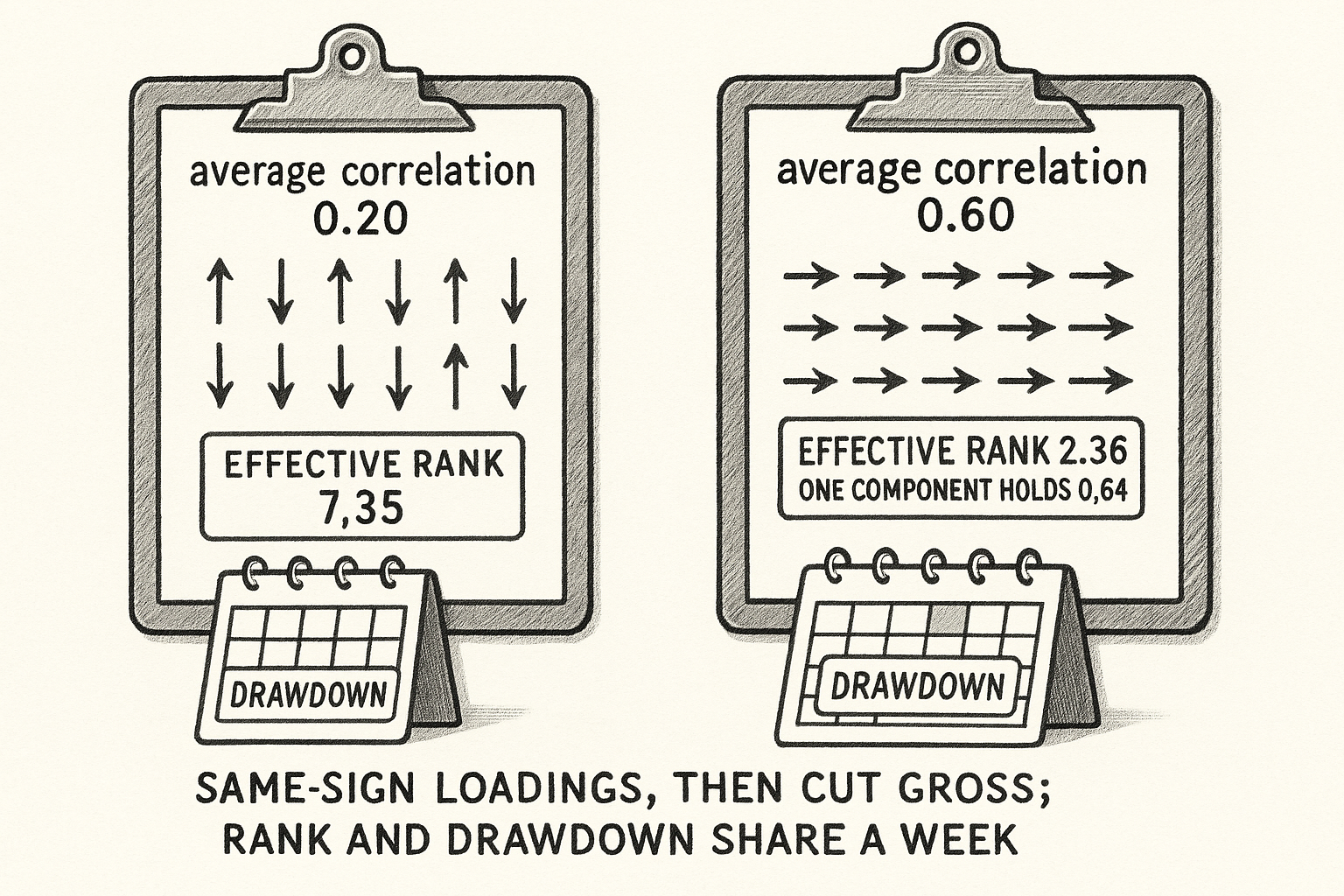
Cross-asset effective rank: ten assets at correlation 0.60 have rank 2.36, and one component holds 0.64 of the variance. Cut gross when its loadings share a sign.

McMillan finds that from 2009 a US stock-bond book needs an 80% stock weight to stay on the return path a 50/50 book had traced before 2000. The correlation between stock and bond returns flipped from positive to negative around 2000 in six of the G7 markets, and it moves back toward positive in the last two years of a sample that ends in December 2023. A negative correlation hedges. A positive correlation puts both positions on one factor, and the variance of the book rises with the covariance term. The object you compute is the effective rank of the correlation matrix of the positions you hold. When that rank falls and the dominant eigenvector carries the same sign on every position, the names in the book are one trade.
Effective rank is how many bets the correlation matrix contains
None of the four source papers prints an effective-rank formula. You build it from the correlation matrix they are already using. Take a matrix in which every diagonal entry is 1 and every off-diagonal entry is the same correlation, call it rho. That matrix equals (1 minus rho) times the identity, plus rho times a matrix of ones. The all-ones vector picks up the eigenvalue 1 plus (N minus 1) times rho. Any vector whose entries sum to zero is wiped out by the ones matrix and keeps the eigenvalue 1 minus rho. There are N minus 1 of those vectors. The eigenvalues sum to N, which is the trace, so the algebra closes.
$$ \lambda_1 = 1 + (N-1)\rho, \qquad \lambda_{2,\ldots,N} = 1 - \rho $$
Lambda-1 is the all-ones direction, the common bet. The other eigenvalues are the leftover directions. Lambda-1 is the largest only when rho is positive. When rho is negative the leftover eigenvalues are larger, and the dominant direction is a spread. The matrix is a valid correlation matrix only when every eigenvalue is non-negative, so rho sits between -1/(N-1) and 1. For ten assets that floor is -1/9, about -0.11. A hedge with a largely negative correlation has to live in a few pairs.
The effective rank is the participation ratio of those eigenvalues. On a correlation matrix the eigenvalues sum to N, so the ratio is N squared over the sum of squared eigenvalues.
$$ \mathrm{PR} = \frac{\left(\sum_{i=1}^{N}\lambda_i\right)^2}{\sum_{i=1}^{N}\lambda_i^2} = \frac{N^2}{\sum_{i=1}^{N}\lambda_i^2} $$
The second equality is the correlation-matrix case. A rank near N means the eigenvalues are close to equal and the names still move on their own. A rank near 1 means one eigenvalue ate the matrix. At rho equal to zero every eigenvalue is 1, the sum of squares is N, and the rank is N. That is the check.
Worked, N equal to 10. At rho equal to 0.20, lambda-1 is 1 plus 9 times 0.20, which is 2.80, and each leftover eigenvalue is 0.80. Squared: 2.80 squared is 7.84, and 0.80 squared is 0.64, so 9 times 0.64 is 5.76. The sum of squares is 13.60. The rank is 100 divided by 13.60, which is 7.35. Ten names, about seven bets. At rho equal to 0.60, lambda-1 is 6.40 and each leftover is 0.40. Squared: 6.40 squared is 40.96, and 0.40 squared is 0.16, so 9 times 0.16 is 1.44. The sum of squares is 42.40. The rank is 100 divided by 42.40, which is 2.36. The same ten names are about two bets. The trace check at rho equal to 0.20 is 2.80 plus 9 times 0.80, which is 10.
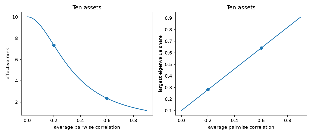
The left panel is the rank. The right panel is the share of the largest eigenvalue. Both curves are the equicorrelation algebra above, computed from the formulas, with no market data in them. The two dots are rho equal to 0.20 and rho equal to 0.60.
The largest share is the bet, and COVOL is what is left after you remove it
The share of the largest eigenvalue is that eigenvalue divided by the sum of the eigenvalues. On a correlation matrix the denominator is N.
$$ \pi_{(1)} = \frac{\lambda_{(1)}}{\sum_{i=1}^{N}\lambda_i} $$
Lambda with a parenthesis is the largest eigenvalue, which equals lambda-1 only when rho is positive. At rho equal to zero the share is 1/N. For ten assets that is 0.10, a tie across every direction. At rho equal to 0.20 the share is 2.80 divided by 10, which is 0.28. At rho equal to 0.60 it is 6.40 divided by 10, which is 0.64. One direction holds about two-thirds of the variance, which is the same fact as the rank falling to 2.36.
Pham, Han, Nguyen, Pham, and Do put the first principal component of 25 cryptocurrency excess returns, the direction of the largest eigenvalue of that covariance, in as the factor in their return regression, their equation (1). They never report that component's variance share. After a GARCH(1,1), which sets today's variance from yesterday's variance and yesterday's squared residual, the standardized residuals still share a volatility shock. The equicorrelation of those squared residuals is 0.043, and their test statistic is 20.67 with a p-value they report as 0. That 0.043 is the correlation of squared residuals after the principal component and the GARCH have already been taken out. Leave it out of the rank formula. The return correlation is the separate series whose slope on squared COVOL is 0.02.
They then fit one positive common-volatility factor, COVOL, whose mean is 1 by construction. Each coin's residual variance is scaled by a loading times that factor.
$$ g_{i,t} = s_i\,(x_t^{\sigma} - 1) + 1 $$
g is the multiplier on coin i's residual variance on day t. s is that coin's loading, estimated once over the sample. x is that day's COVOL. After this factor is removed, the squared-residual equicorrelation falls to 0.0013 and the test statistic falls to 0.635, with a p-value of 0.26. One volatility factor soaks up the co-movement the principal component left behind.
Worked on their own numbers. Bitcoin's loading is 0.2311. On 12 March 2020, COVOL prints 29.06. The gap from the mean of 1 is 28.06. Then 0.2311 times 28.06 is 6.4847, and g is 7.48. The square root of 7.4847 is 2.736, which rounds to 2.74, so the residual shock that day is 2.74 times a normal day in standard-deviation units. The loading is a full-sample constant applied to that day's COVOL. The same day the S&P 500 fell 10%, WTI fell 4.6%, and gold fell 3.6%. Their other COVOL peaks, including the sample maximum of 52.06 on 2 March 2015, land on crypto-specific news while those traditional markets are quiet. A crypto COVOL spike is sometimes the macro factor and sometimes a local one. You do not mark your equity book as collapsed because a coin factor spiked.
On the monthly regression, a one-unit rise in squared COVOL lines up with a 0.02 rise in the average pairwise return correlation that same month, with a lag of the correlation itself in the regression. They do not print the monthly COVOL series beside the daily spike of 29. The paper never puts 29 and 0.02 in one equation. The source may be mixing a daily level with a monthly slope. Leave the two numbers unmultiplied. The coefficient is a same-month association of 0.02 per unit of the squared monthly measure. In the companion volatility regression, squared COVOL has coefficient 0.42 (standard error 0.17) on a broad crypto index's variance shock, and 0.38 in the regression that also includes policy uncertainty, the VIX change, and geopolitical risk. That fuller regression has an R-squared of 21.4%. A fifth of monthly crypto variance, same month.
The old article "The SDF View: One Equation Behind Every Factor Model" writes a pricing kernel on a short list of excess-return factors. A covariance whose largest eigenvalue holds 0.64 of the variance is the risk matrix that makes a one-factor kernel enough. The rank is that statement computed on the book you hold, before anyone names the factor.
A sign flip shows up in portfolio variance
For two assets the eigenvalues are 1 plus rho and 1 minus rho. The rank barely moves when the correlation changes sign at a similar magnitude, and the direction of the large eigenvalue flips.
At rho equal to -0.30 the eigenvalues are 0.70 and 1.30. The sum of squares is 0.49 plus 1.69, which is 2.18, and the rank is 4 divided by 2.18, which is 1.83. The larger eigenvalue, 1.30, belongs to the vector (1, -1). Its share is 1.30 divided by 2, which is 0.65. The dominant direction is the hedge. At rho equal to +0.40 the eigenvalues are 1.40 and 0.60. The sum of squares is 1.96 plus 0.36, which is 2.32, and the rank is 4 divided by 2.32, which is 1.72. The share of the larger one is 0.70, and that eigenvector is (1, 1). The rank moved from 1.83 to 1.72. The dominant loadings changed from opposite signs to the same sign.
McMillan's US three-year rolling correlation has mean -0.01, a minimum of -0.79, and a maximum of 0.65. The values -0.30 and +0.40 sit inside that range. They are worked levels, not dates he singled out. The blue line is a dynamic conditional correlation from a GARCH, Engle's DCC, which updates the correlation from recent residuals. Its US mean is -0.02, its minimum -0.62, and its maximum 0.54. Recompute the orange line. It is a three-year rolling correlation of monthly returns.

Look at the US panel, the bottom one, and follow the orange line at the right edge. It crosses back above zero at the end of the sample. Canada, Germany, and the UK do something similar. France turns up earlier. Italy spends more of the sample positive. Japan goes negative in the first half of the 1990s.
The variance of a two-asset book is the usual weighted sum of variances plus the covariance. McMillan's prose describes that formula. The equation printed in the paper multiplies each variance by the weight 50%, where the squared weight is 0.25, and it adds the correlation in the covariance term where the formula multiplies by the correlation. Those pieces do not add up to the portfolio variance. The printed equation may be wrong. The card is the formula the prose describes.
$$ \sigma_p^2 = w_s^2 \sigma_s^2 + w_b^2 \sigma_b^2 + 2\, w_s\, w_b\, \sigma_s\, \sigma_b\, \rho $$
w is the weight, sigma is the volatility of that leg, and rho is the correlation. With equal weights of one half and equal volatilities sigma, this collapses to sigma-p equal to sigma times the square root of one half times (1 plus rho). Set both volatilities to 10% so the correlation is the only moving part. Bonds are quieter than stocks in a real book; this equal-vol case is the correlation term on its own.
At rho equal to -0.30, the inside of the square root is 0.5 times 0.70, which is 0.35. The square root is 0.5916, and portfolio vol is 5.92%. At rho equal to +0.40, the inside is 0.5 times 1.40, which is 0.70. The square root is 0.8367, and portfolio vol is 8.37%. The second vol is 1.41 times the first. Dividing 5.92 by 8.37 gives 0.71. To hold the old vol you multiply gross by 0.71. Recompute it with your own two volatilities before you touch a live book. A 10% bond vol is a high bond.
McMillan's 65% and 80% stock weights are a different exercise. He fits a trend to the US 50/50 cumulative return through the end of 1999, extrapolates it, and raises the stock weight until the later path matches that line: 65% stocks from 2000 through 2008, 80% from 2009. That fit targets a return path. The 0.71 scale above targets a volatility. In the variance decomposition, the covariance contribution is positive in the first half of the sample and negative in the second half for every G7 market except Italy, where it stays small and positive. A G7 average hides a market that never paid you the hedge.
Community ratio moves; average degree tracks the listing count
Pu, Roberts, Dong, and Zohren learn a graph on 64 futures. An edge means the two contracts have similar momentum features over a lookback. Return correlation is a separate matrix. The old article "Network Momentum as a Cross-Asset Factor" builds the book from that graph. The community ratio, the fraction of contract pairs that still agree with asset-class labels, answers whether those momentum features still respect asset classes.
They print edge sparsity as the fraction of possible pairs that carry an edge.
$$ G_t^{\mathrm{sparse}} = \frac{2\,|\mathcal{E}^{(t)}|}{N_t(N_t-1)} $$
The numerator counts undirected edges twice so it matches the ordered-pair denominator. A larger value is a denser graph. They describe the series as generally below 0.40. If the degree is the unweighted undirected degree, sparsity equals average degree divided by N minus 1. Use that as a check on your own graph. They also say sparsity, average degree, and the clustering coefficient move with the number of contracts in the file. A rising degree follows the universe getting larger.
The community ratio breaks from the listing count. It scores a pair as agreeing with the asset-class partition when two contracts in the same class are linked, or when two contracts in different classes are not linked.
$$ G_t^{\mathrm{community}} = \frac{2\left(\sum_{i,j} 1_{\{A_{ij,t}\neq 0,\, C_i=C_j\}} + \sum_{i,j} 1_{\{A_{ij,t}=0,\, C_i\neq C_j\}}\right)}{N_t(N_t-1)} $$
C is the asset class. They keep this ratio above 0.50 for the whole test, and it drops in 2007-2008. A reading above one half means the class labels still describe most pairs. A drop means momentum features are lining up across classes, and the graph moves toward one feature. That is a collapse of the momentum book. Return correlations are the other matrix.
Degree centralization asks whether those edges concentrate on a few hubs. They print the degree and the average degree. They do not print the centralization ratio. You compute it from their degree.
$$ d_{i,t} = \sum_{j} 1_{\{A_{ij,t}\neq 0\}}, \qquad C_t = \frac{\sum_{i}(d_t^{\max}-d_{i,t})}{(N_t-1)(N_t-2)} $$
The denominator is the value of the numerator on a star, so the ratio runs from 0 to 1. Worked on a toy of four nodes, because their paper never reports the maximum degree and the average alone cannot produce this number. A star has degrees 3, 1, 1, 1. The gaps from the maximum are 0, 2, 2, 2, and the sum is 6. The denominator is 3 times 2, which is 6. Centralization is 1. Equal degrees give a numerator of 0 and a centralization of 0. Their text says the average degree is stable and moves with the number of listed contracts, on a 64-futures universe. A star on 64 nodes has average degree near 2, which is 2 times 63 divided by 64. They never report a degree profile that looks like that star. Centralization, computed from a flat degree profile, sits still while the community ratio moves. Track the community ratio.
On 22 December 2006, a calm date in their telling, equity and fixed-income contracts still share edges. On 5 April 2022, a date whose five-year lookback includes the pandemic and the Ukraine war, those equity-to-bond edges are absent and equities form a tighter cluster. The 2008 low in the community ratio and the April 2022 graph are different shapes. One stress mixes the classes in the momentum features. The other separates equity from bonds and tightens equity on itself. A single rule that raises centralization and cuts every position misses one of these two dates.
The slow statistics coincide with the stress
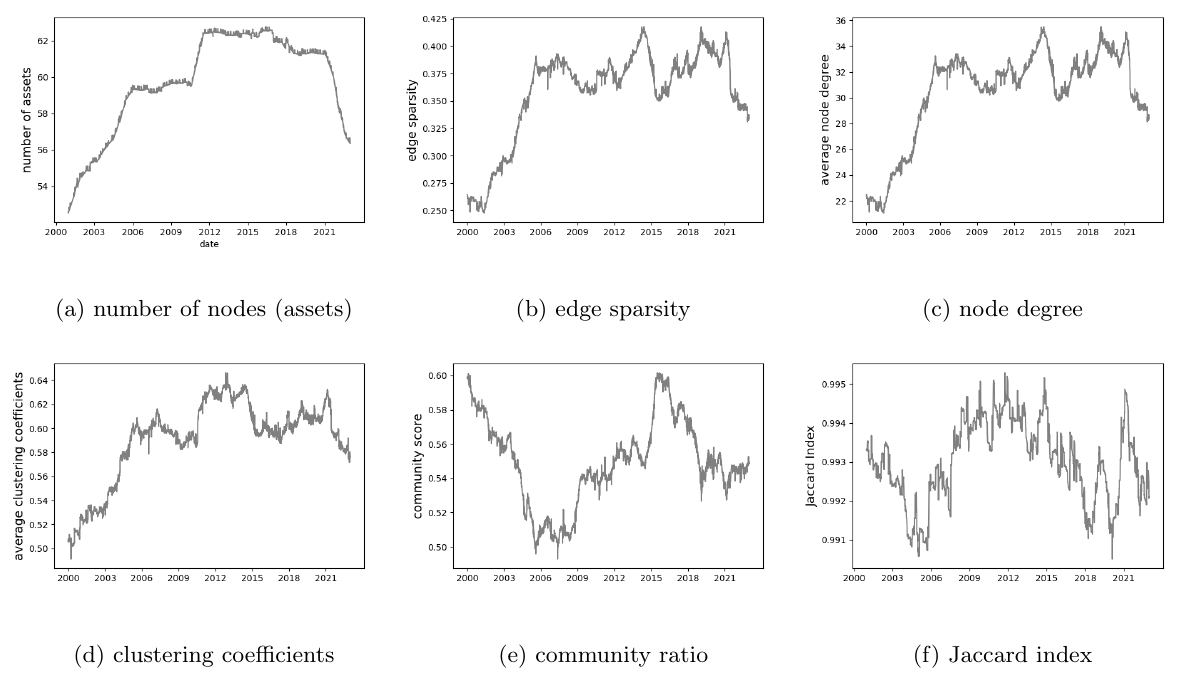
Look at panel (e), the community ratio. The low sits on 2008-2009, with the crisis, while panel (a) shows the contract count still elevated. Panel (f), the Jaccard index of edges kept from one day to the next, stays generally above 0.99 and wiggles in 2008 and again in 2020. A few edges differ from the previous day during the stress. The index stays intact through the prior year.
The performance comparison, on signals scaled to a 15% volatility target, is the full network book against the same book with only within-class edges and only cross-class edges. Sharpes are 1.51, 1.21, and 0.91. Returns are 0.22, 0.18, and 0.13, maximum drawdowns are 0.20, 0.29, and 0.61, and the fraction of days they count as drawdown duration is 6.9%, 9.3%, and 27.3%. The within-class leg and the cross-class leg correlate 0.51, which is why bolting them together beats either leg. The cross-class leg is the one that drops in 2007-2008. The authors read that drop as asset classes behaving differently in a crisis. A return-correlation collapse would have made the classes behave the same way. Their sentence and a diversification-death story are in tension, and the table is what you have: the cross-class momentum leg has the worse drawdown, Sharpe 0.91 against 1.51, maximum drawdown 0.61 against 0.20.
On the raw-signal book, whose no-cost Sharpe they state as 1.36, a 5 basis point cost takes the cost-adjusted Sharpe to -0.67. That 1.36 matches the raw-signal panel. The vol-scaled Sharpe is the 1.51 above. The cost test prices turnover of the momentum signal. A one-time cut in gross is a separate trade, and they do not measure it.
A lead would put the drop before the drawdown. The community-ratio low prints on the crisis years. The COVOL coefficient of 0.02 is a same-month regression. The stock-bond sign change is the regime itself, and a three-year window cannot cross zero until a long stretch of the new regime is already inside it. The one timed lead in these papers is in Easley, O'Hara, Yang, and Zhang. On Binance one-minute bars for five coins, from January 2021 to July 2023, a random forest predicts the sign of the next change in realized volatility at an accuracy of 0.56 to 0.58, depending on a 50-bar or 100-bar lookback. The horizon is 1,500 bars, about one day, chosen so the label does not overlap the feature window. Average accuracy across their labels is 0.53 to 0.54. Skewness sits at 0.50. Mean VPIN, an average of absolute order-flow imbalance scaled by volume, runs from 0.45 to 0.47, against about 0.22 to 0.23 in the E-mini and crude in earlier futures work they cite. The Roll measure is twice the square root of the absolute autocovariance of price changes, a spread proxy from serial correlation. Bitcoin and Ethereum Roll measures and VPINs predict the other three coins. The other coins' features do little for Bitcoin or Ethereum. Splitting the sample on 10 November 2021, the market-cap peak, leaves the accuracy almost unchanged. They say the forest is short of a causal claim. The old article "Crypto Isn't Structurally Alien: Roll/VPIN/Amihud Predict Distribution Shifts" is that one-day forecast: a lead of a volatility sign inside five coins on one exchange. They never test it as a hedge of a multi-asset drawdown.
The rank moves in the same window as the loss. I am against adding risk on a forecast that it will move first. Cut gross when it has moved.
Cut gross when the loadings share a sign
The scale is the vol you were running, at the correlation already in the book, divided by the vol at a wider correlation.
$$ \kappa = \frac{\sigma_p(\rho_{\mathrm{old}})}{\sigma_p(\rho_{\mathrm{wide}})} $$
Multiply gross by kappa. In the equal-vol example, rho of -0.30 against rho of +0.40 gives kappa equal to 0.71. With a real stock vol and a real bond vol the number moves. Recompute the variance card with those vols. The 0.71 belongs to the equal-vol example.
Run two correlation windows. The three-year window is the one McMillan shows, and it is late by construction. A 63-day window moves sooner and jumps around. Acting only when both windows say the correlation has risen, and the dominant eigenvector has the same sign on the positions you are long, is a desk rule. Neither paper tests it. The 63-day length is arbitrary. If the dominant loadings have mixed signs, a hedge is still inside the book, and a flat gross cut throws the hedge out with the bet. If every loading has the same sign, nothing inside the book hedges it. You cut gross, or you buy something that is not in the matrix.
On the momentum graph, turn the cross-class leg down when the community ratio is falling. That is the leg in the comparison above. Leave the within-class leg until its own rank says otherwise. A missing equity-to-bond edge, as on 5 April 2022, is a reason to keep the bond only while the return correlation is still negative. The old article "Stock-Bond Correlation: The Sign Flips and So Do Its Drivers" dates the US move back toward a positive correlation in the last two years of the sample, and 2022 sits in that window. Use the return correlation for the gross cut. Use the community ratio to decide whether the cross-class momentum leg is still a separate signal.
The old article "Good vs Bad COVOL in Crypto: A Common-Volatility Tilt" trades the gap between upside and downside common vol. That tilt sets the sign of the common shock. The gross cut is the separate decision, from the rank and the loadings. Use COVOL as a same-month flag that residual variances have synced, and widen the correlation you feed the risk model by something on the order of the 0.02 coefficient. The daily print of 29 is in different units, as the COVOL section showed.
What these papers leave out is the cost of the cut, the lag of the long window, and the universe. The 5 basis point test above prices turnover of a signal that retrades. A one-time reduction in gross pays the spread and the slippage once, on the day the loadings match, and nobody in these four papers measures that day. Pham and coauthors pick the 25 coins by market cap on 10 April 2024 and keep coins that stayed listed, so the universe looks ahead. Pu and coauthors' contract count moves as the futures file gains and loses names. Easley and coauthors use one exchange and five coins. McMillan uses monthly G7 data with country start dates that differ, the US from 1980. Treat the vol-scaled network Sharpe above as a gross research book on that futures file. The rank is the exposure dial on the book you hold.
KEY POINTS
- Compute effective rank as N squared over the sum of squared correlation eigenvalues. At an average correlation of 0.60, ten assets have effective rank 2.36, and the largest eigenvalue holds 0.64 of the variance.
- On an equal-vol 50/50 book at 10% vol each, correlation of -0.30 gives portfolio vol 5.92%, and correlation of +0.40 gives 8.37%. Multiply gross by 0.71 to hold the old vol. The US three-year rolling correlation itself runs from -0.79 to +0.65.
- Track the community ratio on the momentum graph. Pu, Roberts, Dong, and Zohren keep it above 0.50, and it drops in 2007-2008. Average degree and edge sparsity move with the number of listed contracts.
- The full network book, scaled to 15% vol, has Sharpe 1.51. The cross-class leg has Sharpe 0.91 and maximum drawdown 0.61. Turn that leg down when the community ratio falls.
- Treat a rank drop as a same-window exposure cut. The community-ratio low sits on 2008-2009, and the COVOL correlation coefficient of 0.02 is same-month. The one timed lead is a one-day vol-sign accuracy of 0.56 to 0.58.
References
- The SDF View: One Equation Behind Every Factor Model
- Network Momentum as a Cross-Asset Factor
- Crypto Isn't Structurally Alien: Roll/VPIN/Amihud Predict Distribution Shifts
- Stock-Bond Correlation: The Sign Flips and So Do Its Drivers
- Good vs Bad COVOL in Crypto: A Common-Volatility Tilt
- Stock-Bond Return Correlation: Understanding the Changing Behaviour
- Good versus Bad COVOL in Cryptocurrency Markets: A Measure of Asymmetric Common Volatility
- Network Momentum across Asset Classes
- Microstructure and Market Dynamics in Crypto Markets
A note on AI. The ideas, research, analysis, and conclusions in this article are my own. I use AI tools to help with editing and wordsmithing, because English is not my first language, and I am not shy about that. AI-generated ideas and AI-assisted writing are not the same thing: the first is empty slop from a generic prompt, the second is a tool for communicating years of real research more clearly. Judge the work by its substance, not by whether software helped polish the prose.