10. Cross-Sectional & Factor Investing July 9, 2026 10 min

10.9 The SDF View: One Equation Behind Every Factor Model

Every factor model, from Fama-French to a neural net, is one equation: the SDF. Same skeleton, but the choice of characteristics and weighting function swings out-of-sample Sharpe from 0.45 to 3.4.

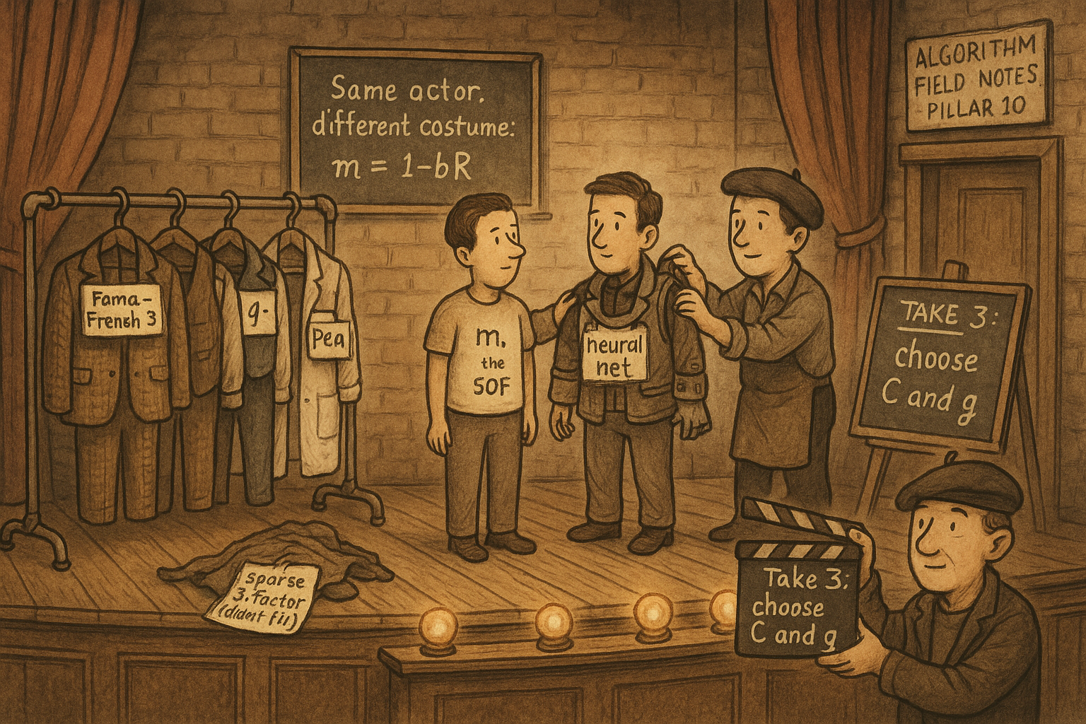
Ask ten quants what a factor model is and you get ten answers: Fama-French three-factor, the q-factor model, a random forest, a neural net, principal components on a thousand characteristics. They sound like rival religions. They are not. Every one of them is the same single equation with different furniture bolted on. That equation is the stochastic discount factor, and once you see it, the factor zoo stops looking like a menagerie and starts looking like one animal wearing costumes.

Chuan Shi's lecture notes lay the frame out cleanly. Write down one pricing object, the SDF, let its portfolio weights be a function of firm characteristics, and every model from a 1990s double sort to a 2024 adversarial network becomes a choice of two things: which characteristics to feed in, and what function turns them into weights. The payoff is not philosophical. On the same test, machine-learning SDF estimators post out-of-sample Sharpe ratios of 3.2 to 3.4 while the Fama-French three-factor model manages 0.45. Seven times the risk-adjusted return from the same equation, just better choices inside it.

The old article "What Is a Factor, Really" defined a factor operationally: an alpha so pervasive you keep re-finding it, so you regress it out before hunting anything new. The old article "What a Factor Actually Is: alpha plus beta-transpose lambda" gave the cross-sectional line every model argues over. This article goes one level deeper, to the object those factor premiums are shadows of. Everything in this pillar is a special case of what follows.

One law: the SDF prices everything

Start with the only assumption that matters, no near-arbitrage. If there is no portfolio out there earning an absurd Sharpe ratio for free, then there exists a single random variable, call it m, that prices every asset at once. The pricing law is that the expected product of m and any asset's excess return is zero. For every asset i, at every date t, the market sets the price so that m and the payoff cancel in expectation. One equation, the whole cross-section.

The trick the modern literature uses is to write m itself as one minus a portfolio of the very returns it prices.

$$ m_{t+1} = 1 - \mathbf{b}_t^\top \mathbf{R}_{t+1}^e, \qquad b_{i,t} = g(\mathbf{c}_{i,t}) $$

Read it slowly. m-sub-t-plus-1 is next period's discount factor. R-e is the vector of excess returns on all N stocks. b-sub-t is a vector of weights, one per stock, and the dot product b-transpose R-e is just the return on a portfolio built with those weights. The second piece is the whole idea: the weight on stock i is not a free parameter, it is a function g of that stock's characteristics c-sub-i-t, its size, its book-to-market, its momentum, its 300 other features. The SDF is a characteristic-weighted portfolio, and g is the recipe that turns a company's traits into how much it belongs in that portfolio.

Work a toy version. Two stocks, weights driven only by book-to-market, and suppose g just copies the value score, so a stock with value score 0.8 gets weight 0.8. If the two stocks return 3% and minus 1% next month, then b-transpose R-e is 0.8 times 3 plus 0.2 times minus 1, which is 2.2%, and m is 1 minus 0.022, or 0.978. The SDF is low in states where the value portfolio pays off. That is the entire content of "value is a factor": the discount factor moves with it.

Collapse the weights into managed portfolios

The function g can be anything, and anything is hard to estimate. So you approximate it as a weighted sum of simpler building blocks, each one a portfolio you can actually form.

$$ m_{t+1} = 1 - \sum_{k=1}^{K} \theta_k \, \tilde{R}_{k,t+1}^e, \qquad \tilde{R}_{k,t+1}^e = \sum_{i=1}^{N} g_k(\mathbf{c}_{i,t})\, R_{i,t+1}^e $$

The inner sum builds factor k: take every stock, weight it by g-sub-k of its characteristics, add up the returns, and you have R-tilde-k, a managed portfolio. The outer sum mixes those K factors with coefficients theta. Those thetas are the SDF loadings, the thing you estimate. This is the unconditional form, and it is where the costumes go on. A sign convention floats around here, some write it with a plus, because the sign gets absorbed into theta, so do not read anything into it.

Now watch every model fall out of this one line. Fama-French three-factor: K is three, the characteristics are market cap and book-to-market, and each g-sub-k is a double portfolio sort into big-small and value-growth buckets. The q-factor model swaps in investment and profitability sorts. Principal-components approaches let the data pick the g-sub-k as eigenvectors of the return covariance. A neural net lets g-sub-k be an arbitrary nonlinear function learned by gradient descent. Same skeleton, different g. The research problem splits exactly two ways: find C, the characteristics worth including, and find g, the function mapping them to weights. The rest is estimation.

The goal also splits, and the split is the whole fight in the field. The traditional academic goal is a parsimonious model that minimizes in-sample pricing errors on a handful of published anomalies. The industry goal is to maximize the out-of-sample Sharpe ratio of the mean-variance-efficient portfolio the SDF implies. Those are not the same target, and optimizing the first has a long history of failing the second.

The scoreboard: same equation, seven times the Sharpe

Here is why the framing earns its keep. Put several choices of C and g on the same out-of-sample test and the spread is enormous.

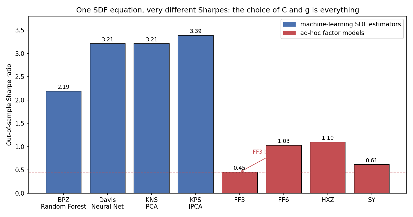
Bar chart of out-of-sample Sharpe ratios, machine-learning SDF estimators near 3.2 to 3.4 versus ad-hoc factor models near 0.45 to 1.1

The textbook models cluster low. Fama-French three-factor posts an out-of-sample Sharpe of 0.45, the six-factor version 1.03, the q-factor model 1.10, the Stambaugh-Yuan mispricing model 0.61. The machine-learning SDF estimators sit in another league: a random forest at 2.19, a neural net at 3.21, a PCA-based model at 3.21, and instrumented PCA (IPCA) at 3.39. IPCA, note, is barely nonlinear, it is essentially a smarter linear factor model that lets loadings depend on characteristics, and it wins the whole table. That detail matters: you do not need a monstrous black box, you need the right characteristics feeding a disciplined g.

None of this is a different equation. It is the same SDF. The three-factor model chose three characteristics and a crude g and left most of the risk-return relationship on the table. The winners chose many characteristics and a g flexible enough to capture nonlinearities and interactions. The equation was never the constraint. The choices were.

Sparsity is the illusion, and priors are the fix

The obvious objection: if more characteristics win, why not dump in everything and let the machine sort it out? Because asset pricing is the worst possible environment for naive machine learning. The signal-to-noise ratio is very low, the number of predictors rivals the number of observations, prediction error feeds straight into portfolio risk rather than staying an abstract statistic, and the data-generating process does not even hold still. Turn a flexible model loose on that and it fits noise with confidence.

Two disciplines rescue it, and they pull in opposite directions from the old "keep it simple" instinct. First, sparsity is a myth here. The illusion of sparsity result shows that cross-sectional return prediction does not collapse to three or five true factors. Many characteristics carry information, they are correlated, and model uncertainty is large, so throwing away all but a few costs you out-of-sample. Second, you cannot just estimate freely, you need an economic prior. The figure below, from the shrinking-the-cross-section work, plots the sweet spot: out-of-sample performance is highest when you use a large number of nonzero coefficients and pair it with a prior of the right strength.

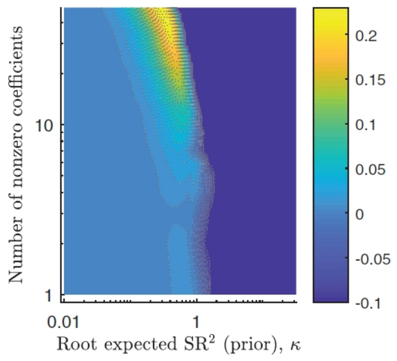
Contour plot of out-of-sample performance against prior strength and number of nonzero coefficients, peaking with many coefficients and a moderate prior

The bright region sits high on the vertical axis, many characteristics, not down at the bottom where sparse models live. But it also needs the prior dialed in along the horizontal axis. Too weak a prior and you overfit, too strong and you shrink real signal to zero. This is where the SDF view repays you again: the natural prior comes from theory. Under no near-arbitrage, the factors that carry high risk premiums must also be the ones that drive how stocks move together. That is not a soft suggestion, it is a testable restriction that tells the estimator where to look, and it is exactly the economic prior the plan for this pillar keeps insisting on.

The prior, made concrete: ridge is Bayesian shrinkage

"Impose an economic prior" sounds vague until you write the estimator. The cleanest case is ridge regression, and its whole appeal is that it is Bayesian shrinkage wearing a linear-algebra disguise.

$$ \hat{\boldsymbol{\theta}} = \left( \mathbf{X}^\top \mathbf{X} + \frac{\sigma^2}{\sigma_g^2}\,\mathbf{I} \right)^{-1} \mathbf{X}^\top \mathbf{y} $$

X is the matrix of factor returns, y the thing you are pricing, and the term added inside the inverse is the whole story. Ordinary least squares is what you get when that term is zero. The ratio sigma-squared over sigma-g-squared is the noise variance divided by your prior variance on the coefficients. When you believe the true loadings are small (small sigma-g), that ratio is large, and it pulls the estimates hard toward zero. When you are confident the data is clean (small sigma-squared) it barely nudges them. A tight prior is literally a big number added to the diagonal.

Put numbers on it. Say the noise variance is 4 and your prior variance on the coefficients is 1, so the penalty is 4 over 1, which is 4. A raw signal that OLS would estimate near, say, 1.0 gets shrunk down toward roughly 1 over 1 plus 4, about 0.2, in the simplest one-regressor case. You gave up unbiasedness on purpose and bought a large cut in variance, and out-of-sample that trade wins. The deck's own experiments show ridge beating OLS on both out-of-sample R-squared and Sharpe ratio for exactly this reason. Overfitting, in one line, is placing too much weight on this dataset and too little on prior experience, and in investing, ignoring prior experience is how you blow up.

The same skeleton, from double sorts to trees to GANs

Because everything is a choice of g, the frontier is just more expressive g functions. One line of work builds g as a decision tree: split the universe by size, then by value, then by size again, and each leaf becomes a portfolio. The picture is a literal tree.

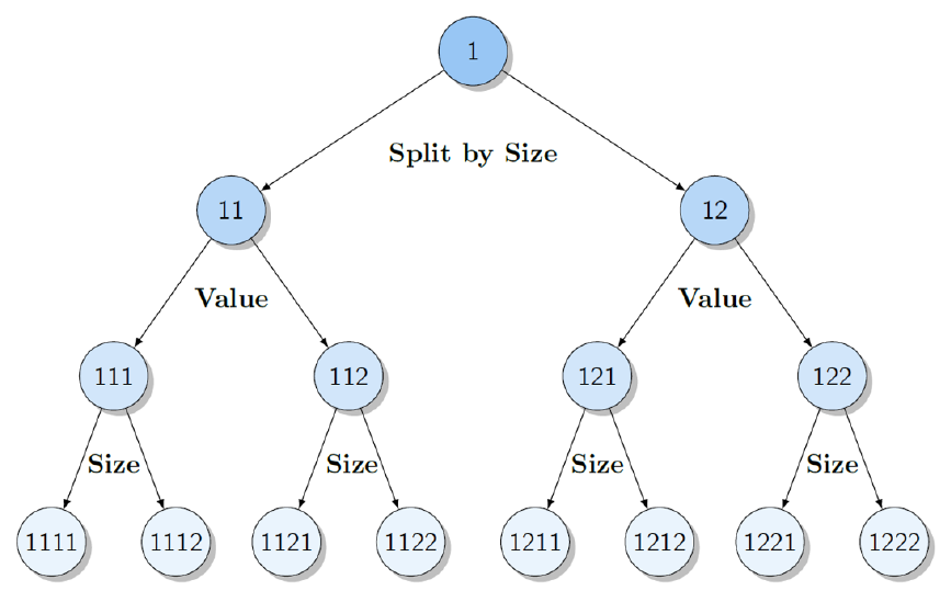
Decision tree splitting stocks first by size, then value, then size again, with each leaf node forming a portfolio

A Fama-French double sort is just this tree pruned to two levels. Grow it deeper and let the estimator shrink both the expected returns and the covariance of the resulting factors, and you get a far richer SDF from the same equation. Push further and g becomes an adversarial network: one network builds the SDF to minimize pricing errors while a second network hunts for the portfolios where the SDF fails worst, and they fight until the SDF prices even the hardest test assets. The no-near-arbitrage condition itself becomes the loss function. Different g, same m. The genealogy runs straight from a hand-drawn double sort to a neural net, and nothing in between changed the underlying law.

Where this connects

The SDF is the equation the rest of this pillar keeps circling. The cross-sectional line from the old article "What a Factor Actually Is: alpha plus beta-transpose lambda" is what you get when you take the SDF's implications for expected returns, so alpha and the premium lambda are downstream of m, not separate objects. The factor-premium fights, the tests of whether a set of alphas is jointly zero, the second-pass premium estimates, all of them are questions about the theta coefficients and the choice of g in this one framework. And the t-cutoff debate from the reckoning articles is the "find C" half of the problem: which characteristics survive honest testing, given that true factors attenuate roughly 36% out of sample.

There is also a geometric reading worth flagging for the information-geometry thread elsewhere in the project. The set of SDFs consistent with no-arbitrage is a convex region, choosing a model is picking a point in it, and the mean-variance-efficient portfolio the SDF implies is the projection that maximizes squared Sharpe. Priors are curvature imposed on that space, and shrinkage is a walk back toward the prior's center. That is speculative framing on my part, not from the source, but the SDF is the natural object to hang it on. Name the one equation, and every model in the zoo becomes a coordinate rather than a creature.

KEY POINTS

Under no near-arbitrage there is a single stochastic discount factor m that prices every asset at once, and its defining property is that the expected product of m and any excess return is zero. Every factor model is a way of writing m.
Write m as one minus a characteristic-weighted portfolio, m equals 1 minus b-transpose R-e with the weight b on each stock a function g of its characteristics. The SDF is just a portfolio whose weights are learned from firm traits.
Approximating g by a sum of managed portfolios turns the model into m equals 1 minus a sum of theta-k times factor-k. Fama-French, q-factor, PCA, and neural-net models are all this one equation with different characteristics C and different functions g.
On the same out-of-sample test, machine-learning SDF estimators hit Sharpe ratios of 3.2 to 3.4 (IPCA 3.39, neural net 3.21) versus 0.45 for Fama-French three-factor. The equation is identical, the choices of C and g are not.
Sparsity is an illusion in the cross-section: many characteristics carry information, so sparse three-to-five-factor models leave performance on the table. Best out-of-sample results use many coefficients plus a well-calibrated prior.
Economic priors are not optional. Ridge regression is Bayesian shrinkage, adding noise-over-prior-variance to the diagonal, and no-near-arbitrage supplies the key restriction: high-premium factors must also drive comovement.
The frontier is just more expressive g functions, from double sorts to decision trees to adversarial networks that turn the no-arbitrage condition into a loss. Same skeleton throughout.

References

- Common Risk Factors in the Returns on Stocks and Bonds (Fama and French, 1993)
- Interpreting Factor Models (Kozak, Nagel, and Santosh, 2018)
- Shrinking the Cross-Section (Kozak, Nagel, and Santosh, 2020)
- Empirical Asset Pricing via Machine Learning (Gu, Kelly, and Xiu, 2020)
- Characteristics Are Covariances: A Unified Model of Risk and Return (Kelly, Pruitt, and Su, 2019)
- Deep Learning in Asset Pricing (Chen, Pelger, and Zhu, 2024)
- Forest Through the Trees: Building Cross-Sections of Asset Returns (Bryzgalova, Pelger, and Zhu)
- Economic Predictions with Big Data: The Illusion of Sparsity (Giannone, Lenza, and Primiceri, 2021)
- The Factor Model Failure Puzzle (Baba-Yara, Boyer, and Davis)
- A Forward Looking View of Factor Investing (Shi, 2024)
A note on AI. The ideas, research, analysis, and conclusions in this article are my own. I use AI tools to help with editing and wordsmithing, because English is not my first language, and I am not shy about that. AI-generated ideas and AI-assisted writing are not the same thing: the first is empty slop from a generic prompt, the second is a tool for communicating years of real research more clearly. Judge the work by its substance, not by whether software helped polish the prose.