10.11 Is Value Dead? The Revaluation Decomposition

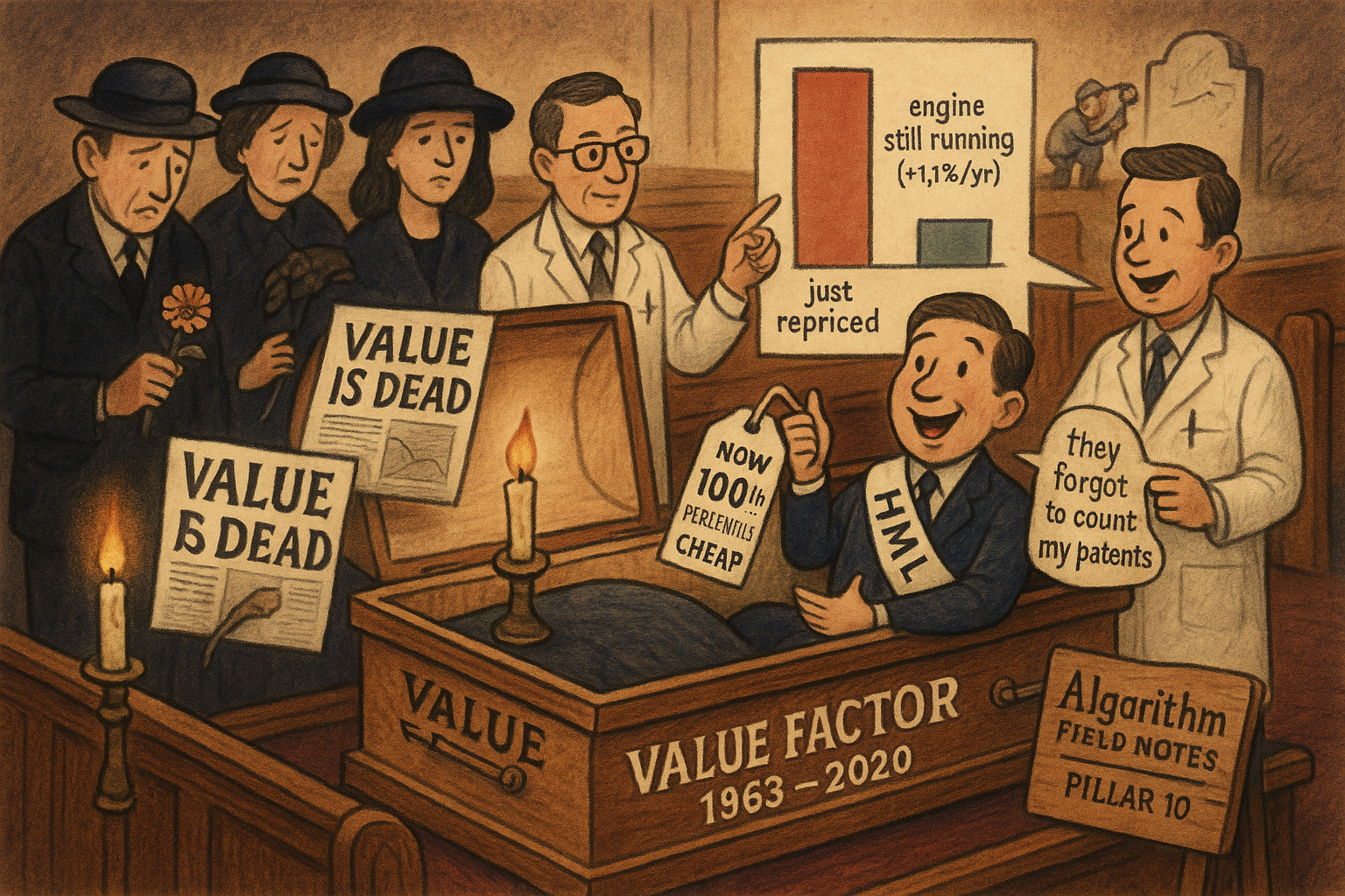
By the middle of 2020 the obituaries were written. The classic value factor, long cheap stocks and short expensive ones, had lost about 55% from its December 2006 peak, a drawdown that ran more than thirteen years. Every quant who had loaded up on book-to-market was underwater for a decade, and the natural conclusion was that the world had changed, the trade was arbitraged away, and value was structurally dead. That conclusion is the expensive one, and it is usually wrong, because it confuses a factor getting cheaper with a factor stopping working.

Arnott, Harvey, Kalesnik and Linnainmaa took the drawdown apart into its moving pieces and found something the death narrative cannot survive. The engine that generates the value premium, the part that comes from cheap stocks staying cheap and paying you income while they do, never stopped running. It contributed a positive 1.1% a year even through the worst stretch. What sank the factor was a separate term: the price gap between value and growth stocks blew out to the widest it had ever been, a 100th-percentile spread. That is a valuation move, and valuation moves mean-revert. The factor was not dying, it was going on sale.

This is the empirical version of two arguments made before. The old article "Why Systems Work Until They Don't" laid out how every strategy decays and how to tell decay from noise. The old article "When to Switch Off a Trading System" built the kill rule: hold inside the envelope, cut on a high-percentile breach, and separate a statistical breach from a structural one. Value in 2020 is the textbook case where getting that distinction wrong would have cost you the recovery.

Split the return into what lasts and what mean-reverts

Start with the accounting identity for a portfolio's log return over one period. Whatever you earn comes from the price moving plus the dividend you collected.

$$ \log(1 + r_t) = \log\!\left(\frac{P_{t^-}}{P_{t-1}}\right) + \log\!\left(1 + \frac{D_{t^-}}{P_{t^-}}\right) $$

P is the portfolio's market value and D the dividend, with t-minus meaning the old portfolio carried to time t before rebalancing. The first term is the capital gain, the second the dividend yield. True so far but useless, because the price move mixes two completely different things: the company genuinely getting more valuable, and the market simply paying a higher multiple for the same book value. You need to separate those, so Arnott and coauthors add and subtract price-to-book terms to break the return into three named pieces.

$$ \log(1 + r_t) = \underbrace{\left[\log\tfrac{P_t^+}{B_t^+} - \log\tfrac{P_{t-1}}{B_{t-1}}\right]}_{\text{revaluation}} + \underbrace{\left[\log\tfrac{P_{t^-}}{B_{t^-}} - \log\tfrac{P_t^+}{B_t^+}\right]}_{\text{migration}} + \underbrace{\left[\log\tfrac{B_{t^-}}{B_{t-1}} + \log\!\left(1 + \tfrac{D_{t^-}}{P_{t^-}}\right)\right]}_{\text{income yield}} $$

Read the three pieces. B is book value, and a superscript plus marks the freshly rebalanced portfolio formed at time t, while t-minus marks the old portfolio drifting into time t. Revaluation is the change in the portfolio's price-to-book multiple across the period, pure repricing. Migration is the jump when you rebalance, capturing the value premium harvested as cheap stocks get repriced upward and graduate out of the portfolio, which Fama and French named the migration effect. Income yield is book-value growth plus dividends, the intrinsic accumulation. Group them and the split that matters falls out: revaluation is the mean-reverting part that should wobble around zero over the long run, while migration plus income yield is the structural premium, the durable payment for holding cheap stocks.

The decomposition verdict: a repricing, not a death

Run the HML factor through this and the death narrative collapses.

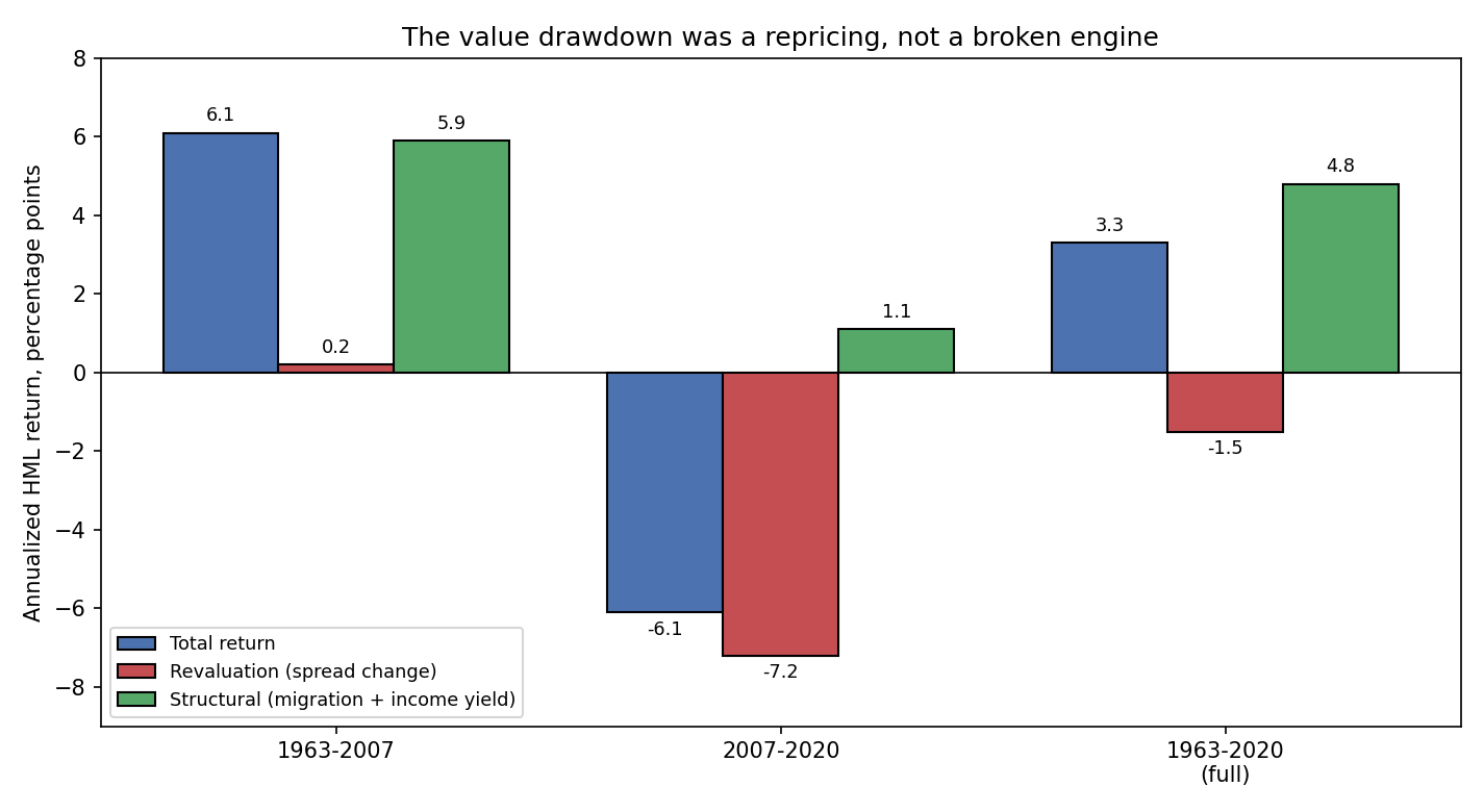
From 1963 to 2007 the factor earned 6.1% a year, and it was almost all structural, 5.9% of it, with revaluation contributing a trivial 0.2%. That is what a working factor looks like: the return comes from the durable engine, not from multiples drifting. Now the crisis window. From July 2007 to June 2020 the factor lost 6.1% a year, and the revaluation term was minus 7.2%. The structural premium over the same stretch stayed positive at plus 1.1%. Read that again. Cheap stocks kept paying the premium while their price relative to growth stocks cratered. The entire loss, and then some, was the value-growth spread widening. Over the full 1963 to 2020 span the structural premium is a healthy 4.8% a year and revaluation is a small negative 1.5%, exactly the near-zero long-run behavior the theory predicts.

The valuation evidence backs it up hard. Asness measured the price-to-book spread between cheap and expensive stocks and found it at the 100th percentile of its entire history in early 2020, more than four standard deviations above the median. Strip out technology, media and telecom, drop the megacaps, drop the 10% most expensive stocks, hold industries neutral, and it stays pinned near the 100th percentile. This was not one bubble sector dragging the number. Value stocks were categorically, broadly, historically cheap relative to growth. A spread that wide is a coiled spring, not a tombstone.

Book value forgot about intangibles

There is a real problem underneath the repricing, and it is not that value stopped working. It is that the ruler got worse. Book value was designed for a world of factories and inventory, and it quietly expenses the things that now build the most corporate value: research and development, brand, software, patents. A firm that pours money into R&D looks like it has thin book value and gets misclassified as expensive, when economically it may be the cheap one.

Arnott and coauthors rebuild the value signal by capitalizing intangibles into book value, producing an intangibles-adjusted factor, iHML.

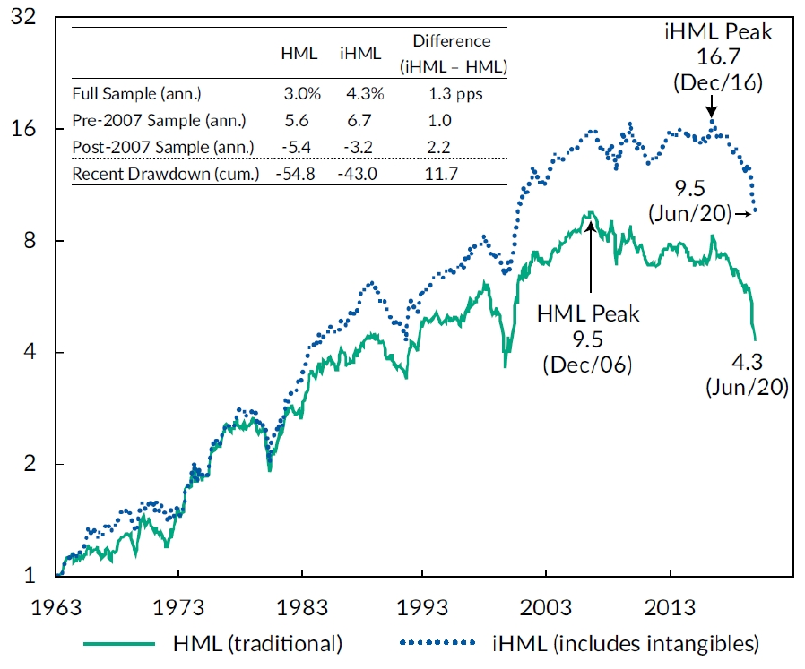
The intangibles version wins across every window. Full sample it earns 4.3% a year against traditional HML's 3.0%. Through the post-2007 drawdown it still lost, but only minus 3.2% a year versus minus 5.4%, and its cumulative drawdown was minus 43% against minus 55%. Better, not saved. iHML peaked in December 2016 and then fell too, because the same valuation-spread blowout hit it. So the two findings stack: the book-value ruler is genuinely outdated and fixing it helps, and on top of that the whole value complex got repriced to an extreme. One is a measurement fix, the other is a mean-reverting cheapness. Neither is death.

Was a 55% drawdown even surprising

Before killing a strategy you owe it one question: is this loss inside the range the strategy could always have produced. The way to answer is a block bootstrap, resampling historical returns in six-month blocks to preserve their autocorrelation, using only pre-2007 data so the recent drawdown does not contaminate the distribution, then reading where the realized loss falls.

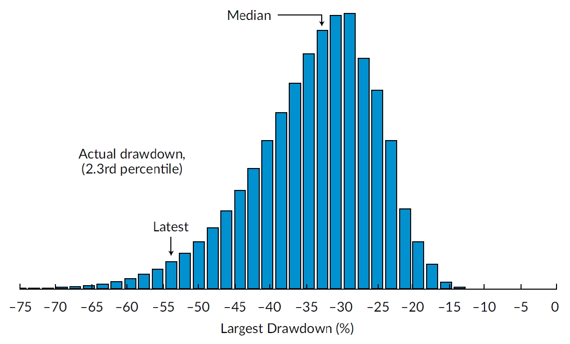
The median simulated worst drawdown is around 32%. The realized drawdown lands at roughly the 2.3rd percentile, deep in the left tail but not off the chart. This is the operational lesson from the old article "When to Switch Off a Trading System" made concrete. A 2.3rd-percentile event is rare, so a disciplined trader cuts risk on a breach that extreme, but it is not proof the edge is gone, because a healthy strategy visits its 2nd percentile roughly one time in forty-something. The mistake is treating a tail draw as a structural break when your own pre-crisis data said such draws were possible. And because the block bootstrap used data ending in 2006, it if anything understated the true odds. The drawdown was ugly and legal at the same time.

The honest kill test: update, do not react

None of this means you hold a dying factor forever out of stubbornness. It means you decide with a rule, not a mood, and the right rule is Bayesian. You start with a prior belief about the factor's premium, you observe a run of recent returns, and you blend the two in proportion to how precise each one is.

$$ \mu_p = \frac{\text{se}^2}{\sigma^2 + \text{se}^2}\,\mu + \frac{\sigma^2}{\sigma^2 + \text{se}^2}\,\bar{r}, \qquad \sigma_p^2 = \left(\frac{1}{\sigma^2} + \frac{1}{\text{se}^2}\right)^{-1} $$

Here mu and sigma are the prior mean and standard deviation of the factor's expected return, r-bar and se are the sample mean and its standard error from recent data, and mu-p and sigma-p are the posterior. The posterior mean is a precision-weighted average: the noisier the recent sample, the less it moves your belief. Then you judge failure by the posterior t-statistic, mu-p divided by sigma-p, not by the raw bad run.

Work it. Say your prior on a monthly value premium is a mean of 0.40% with a standard deviation of 0.20%, so the prior variance is 0.04. A grim recent stretch prints a sample mean of minus 0.50% with a standard error of 0.30%, so its variance is 0.09. The weight on the prior is 0.09 divided by 0.13, about 0.69, and the weight on the data is 0.04 divided by 0.13, about 0.31. The posterior mean is 0.69 times 0.40 plus 0.31 times minus 0.50, which is 0.12% a month, still positive. The posterior variance is one over the sum of 25 and 11.1, about 0.028, so the posterior standard deviation is 0.17% and the t-statistic is roughly 0.7. The verdict is not "dead," it is "shrunk and no longer significant, keep it small and keep watching." That is a decision, and it is the opposite of panic-selling the bottom.

Where this connects

The value debate is the cleanest live example of the decay-versus-noise problem from the old article "Why Systems Work Until They Don't." Four decay mechanisms exist, crowding, regime drift, microstructure change, and capacity saturation, and each has a fingerprint. The 2007 to 2020 value drawdown matched none of them. Its fingerprint was a widening valuation spread with an intact structural premium, which is the signature of a repricing, and repricings are the one kind of drawdown that predicts higher future returns rather than lower. Confuse it with genuine decay and you commit the exact error the old article "When to Switch Off a Trading System" warns is most common and most expensive: quitting inside the envelope and missing the recovery.

Two cautions keep this from becoming a blank check for stubbornness. The decomposition is an attribution done with hindsight, and knowing the loss was revaluation does not tell you when the spread reverts, only that its expected long-run contribution is near zero. And the same accounting that exonerates traditional book value also indicts it, so if your value signal ignores intangibles you are carrying a measurement bug regardless of the spread. The lesson is not "value can never die." It is that death and cheapness leave different fingerprints, and you owe every strategy a decomposition and a bootstrap before you write its obituary.

KEY POINTS

• The classic value factor lost about 55% from December 2006 to June 2020, prompting widespread claims that value was structurally dead.
• Decomposing HML into revaluation, migration, and income yield shows the structural premium (migration plus income yield) stayed positive even in the crisis, at plus 1.1% a year, while revaluation of minus 7.2% a year drove the entire loss.
• Revaluation is the mean-reverting price-multiple term that should hover near zero long-run, and over 1963 to 2020 it was just minus 1.5% while the structural premium was a healthy 4.8%. The engine never broke.
• The value-growth valuation spread hit the 100th percentile of its history, over four standard deviations above median, and stayed extreme after removing tech, megacaps, the priciest names, and industry effects. That is a coiled spring, not a tombstone.
• Book value ignores intangibles like R&D and brand, misclassifying research-heavy firms. Capitalizing intangibles into iHML beats traditional HML in every window, 4.3% versus 3.0% full sample, though it too fell in the spread blowout.
• A block bootstrap on pre-2007 data puts the realized drawdown at roughly the 2.3rd percentile: a deep tail event, but one the strategy's own history said was possible, not proof of a broken edge.
• Judge factor death with a Bayesian update, blending prior and recent sample by precision and testing the posterior t-statistic, rather than reacting to a raw bad run. A grim stretch can leave the posterior positive but shrunk, which argues for smaller size, not abandonment.

References

• Reports of Value's Death May Be Greatly Exaggerated (Arnott, Harvey, Kalesnik, and Linnainmaa, 2021)
• Is (Systematic) Value Investing Dead? (Asness, 2020)
• The Quant Crisis of 2018-2020: Cornered by Big Growth (Blitz, 2021)
• A Five-Factor Asset Pricing Model (Fama and French, 2015)
• The History of the Cross-Section of Stock Returns (Linnainmaa and Roberts, 2018)
• Market Efficiency in the Age of Big Data (Martin and Nagel, 2022)
• Factor Failure (Shi, 2024)