10. Cross-Sectional & Factor Investing July 9, 2026 9 min

10.12 Factor Timing Mostly Fails

Value, momentum, volatility, and sentiment timing all lost to a plain equal-weight factor basket in China. Theory says timing is huge; estimation error eats it. Trust the plateau, not the peak.

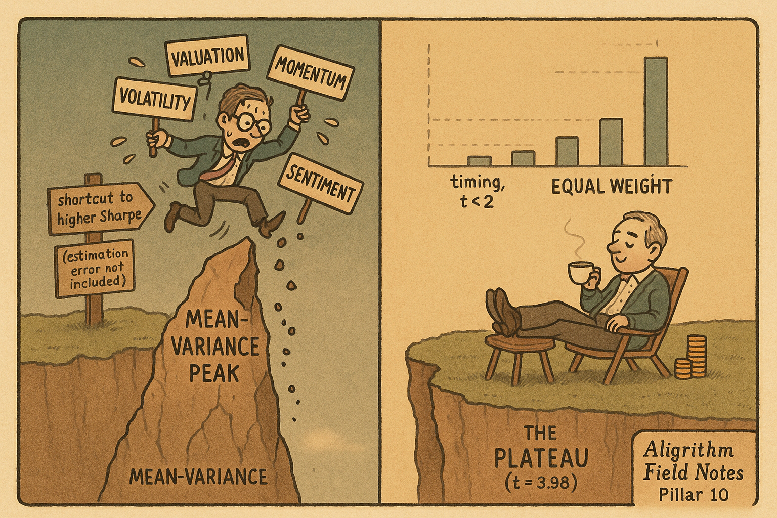
Factor timing is the seductive idea that you can do better than holding a basket of factors: lean into value when value looks cheap, load momentum when momentum is running, cut a factor when its volatility spikes. Every one of those moves has a tidy formula and a plausible story. And when you run them out of sample on a clean universe, almost all of them lose to the dumbest thing you could have done, which is hold every factor in equal weight and never touch it again.

That is the honest version, and it is not a rounding error. Chuan Shi ran the four classic timing signals, valuation spread, factor momentum, factor volatility, and investor sentiment, on the Chinese market from 2000 to 2020, and none of them beat an equal-weighted seven-factor portfolio at any horizon he tried. The equal-weight benchmark itself was real, earning 0.27% a month over the market with a Newey-West t-statistic of 3.98. The timing overlays added nothing on top. Meanwhile there is a genuine theoretical argument, from Haddad, Kozak and Santosh, that timing should matter enormously. Reconciling those two facts is the whole article, and the resolution is the same lesson the old article "Collinearity in Parameter Sweeps: Plateaus, Not Peaks" taught for backtests: robust edges live on wide plateaus, and factor timing is mostly an attempt to stand on a sharp peak that estimation error knocks you off of.

The four timing recipes, and their formulas

Start with valuation timing, the most respectable of the four. You measure each factor's value spread, the valuation of its long leg minus its short leg, and you overweight a factor when its own spread is wide relative to its history. The key discipline is that you compare a factor to itself, never across factors, because every factor lives in its own valuation range.

$$ w_{kt}^{\text{raw}} = 1 + \frac{VS_{kt} - VS_{kt}^{\text{mean}}}{VS_{kt}^{\text{max}} - VS_{kt}^{\text{min}}}, \qquad w_{kt} = \frac{w_{kt}^{\text{raw}}}{\sum_{j=1}^{K} w_{jt}^{\text{raw}}} $$

VS-kt is factor k's value spread now, and the mean, max and min are taken over its own trailing window of T months. The raw weight is a number near 1 that rises above 1 when the factor is cheap relative to its own past and falls below 1 when it is expensive, and then you normalize the raw weights across the K factors so they sum to one. Work a number. Suppose value's spread today sits at 0.8, its trailing mean is 0.5, its max is 1.0 and its min is 0.2. The raw weight is 1 plus (0.8 minus 0.5) over (1.0 minus 0.2), which is 1 plus 0.3 over 0.8, or 1.375. A factor trading at its historical median gets exactly 1.0, and one at its cheapest gets close to 2.0. Tidy. The problem is not the recipe, it is that when Shi actually traded it in China the excess return over equal weight was negative at every lookback from 24 to 60 months, the least bad being minus 0.03% a month with a t-statistic of minus 0.53.

Factor momentum is the second recipe and needs no calculus. Rank the K factors by their trailing twelve-month return, hand the best factor a score of K, the next K minus 1, on down to 1 for the worst, and normalize those scores into weights. It is a winner-loser bet on factors themselves. Sentiment timing is the fourth: build an index from five gauges, the ratio of upside to downside volatility, turnover, the futures basis, new-account growth, and margin-balance growth, each turned into a rolling 252-day percentile, then average them and split into high and low sentiment states. In the Chinese data only momentum and growth factors even showed a statistically detectable sentiment dependence, and timing on it still did not beat equal weight.

Volatility timing, and the correlation that guts it

The third recipe is inverse-volatility weighting. Give each factor a weight proportional to the reciprocal of its own volatility, so the calm factors get more capital and the wild ones get less, which lowers total portfolio volatility.

$$ w_k = \frac{1/\sigma_k}{\sum_{j=1}^{K} 1/\sigma_j} $$

Sigma-k is factor k's return volatility. If three factors have volatilities of 2%, 3% and 6% a month, their reciprocals are 0.50, 0.33 and 0.167, summing to 1.0, so the weights are 0.50, 0.33 and 0.167. The low-vol factor gets triple the weight of the high-vol one. Sensible in isolation, and it is genuinely a risk-reduction tool. But as a timing signal it is largely dead on arrival, because factor volatilities are not independent. Kapadia, Linn and Paye showed factor vols move together, and Shi confirms it: the four style factors in the Chinese five-factor model have an average pairwise volatility correlation of 0.65, and across 92 factors the average is still 0.55. When every factor gets more volatile at the same time, tilting toward whichever is momentarily calmer is noise, not information. Traded in China, volatility timing produced negative excess returns over equal weight at every horizon, none significant.

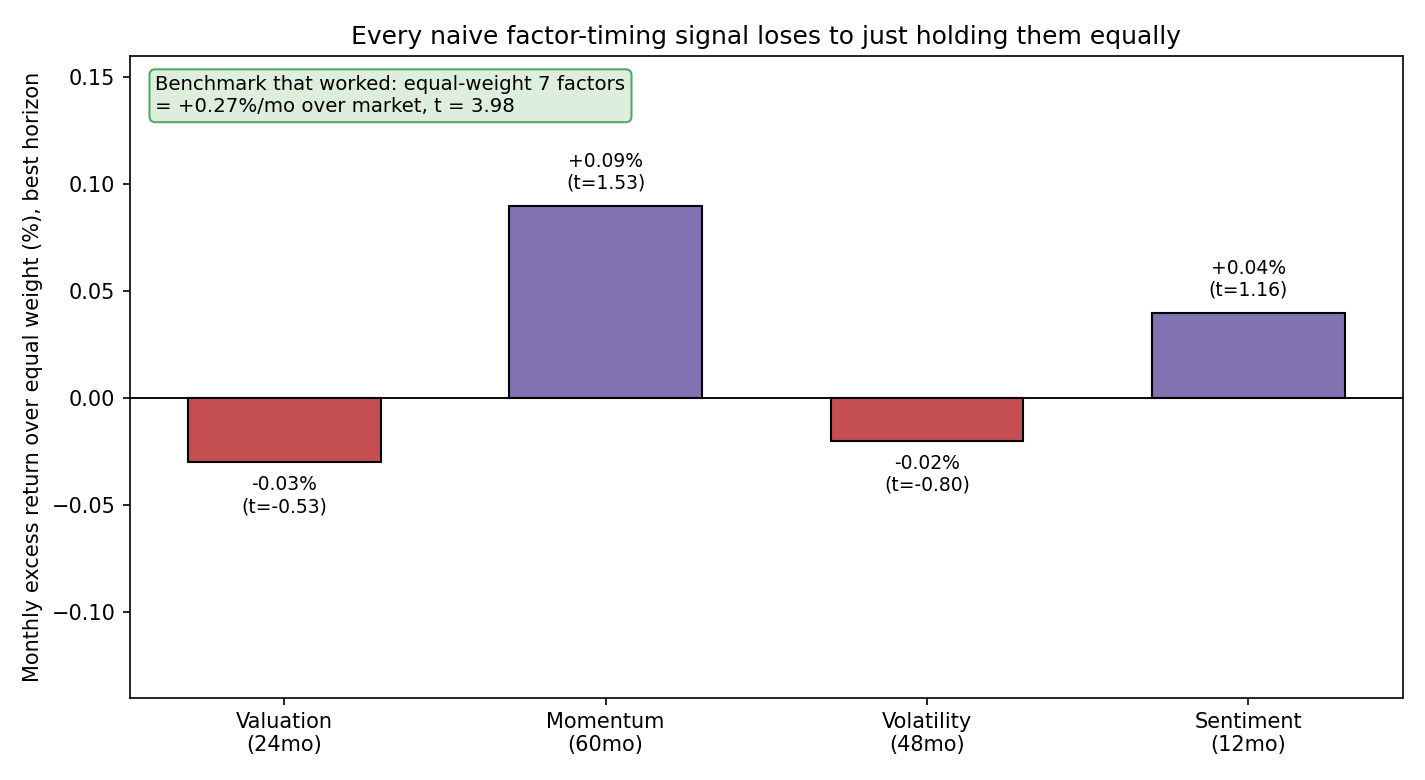
Bar chart of monthly excess return over equal weight for valuation, momentum, volatility, and sentiment timing in China, all with t-statistics below 2, against a note that equal weight itself earned 0.27 percent per month at t equals 3.98

Line the four up and the verdict is blunt. Even choosing the single most favorable lookback for each signal, the steelman case, not one clears a t-statistic of 2. The honest read is not that these signals contain zero information ever, it is that the information is too weak and too correlated to survive real trading once you already hold the factors equally.

The theory says timing should be a big deal

Here is the twist that keeps factor timing alive as a research program. Asset pricing says a stochastic discount factor prices everything, and you can write it as one minus a loadings vector times the surprise in factor returns.

$$ m_{t+1} = 1 - \delta_t^\top \big(f_{t+1} - \mathbb{E}_t[f_{t+1}]\big), \qquad \delta_t = \Sigma_{f,t}^{-1}\, \mathbb{E}_t[f_{t+1}] $$

Here f-t-plus-1 is the vector of factor returns, E-t of f is what you expected given today's information, delta-t is the SDF's loadings, and Sigma-f-t is the conditional covariance of the factors. The optimal loadings are the inverse conditional covariance times the conditional expected returns, which is just the mean-variance efficient weights computed with time-varying inputs. The instant you let E-t of f move over time, you are doing factor timing, so timing is not some optional overlay, it sits inside the definition of the efficient portfolio. And Hansen and Jagannathan proved the maximum attainable Sharpe ratio is bounded by the variance of the SDF, which means anything that raises the SDF's variance raises the ceiling on how good a portfolio can be. Haddad and coauthors measured exactly that: moving from static factor investing to full factor timing lifted the average conditional SDF variance from 1.67 to 2.96, nearly doubling the theoretical Sharpe ceiling. On paper, timing is worth a fortune.

Why the fortune does not show up in your account

The reconciliation is that the predictable part of factor returns is concentrated in a few big dimensions, and everything else is noise you cannot trade. Haddad, Kozak and Santosh ran principal components on fifty anomaly portfolios. The first component alone explains 25.8% of the variance and the first five together explain 60%. Then they asked which components are actually forecastable using their own book-to-market spreads, and the answer is the dominant ones, not the obscure ones.

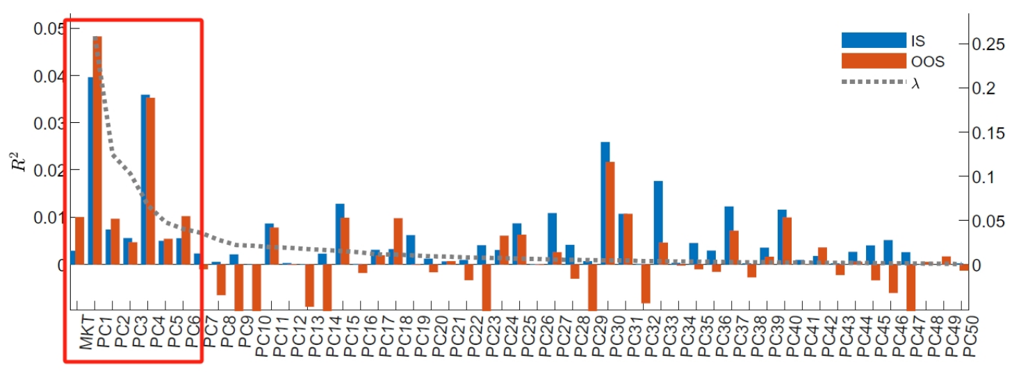
Bar chart of in-sample and out-of-sample R-squared for predicting each of fifty principal components with its own book-to-market ratio, with the first few components boxed as the only ones showing meaningful out-of-sample predictability

The big components, PC1 and PC4, show out-of-sample monthly R-squared of 4.82% and 3.52%, real and tradeable. The long tail of small components has R-squared indistinguishable from zero and often negative out of sample. This is the surprise the original authors emphasized, and it inverts the folk wisdom. The common intuition is that you time individual boutique factors on their own momentum or sentiment. The data says the only reliably timeable object is the handful of dominant common components, timed by valuation. That is why Shi's individual-factor timing in China fails while Haddad's "anomaly timing" of the big US components earns a positive out-of-sample information ratio of 0.60, against minus 0.64 for naive market timing. Timing works, narrowly, exactly where the naive practitioner is not looking.

The plateau beats the peak

Now connect it to allocation, because the failure of timing is really the failure of precision. The mean-variance efficient portfolio is weights proportional to inverse covariance times expected returns, and it delivers the maximum Sharpe ratio if your inputs are right. They never are. Shi says it plainly: the method is highly sensitive to its inputs and estimating expected returns and covariances ex ante is the hard part. So look at what happens when you actually trade the fancy optimizer against the dumb ones.

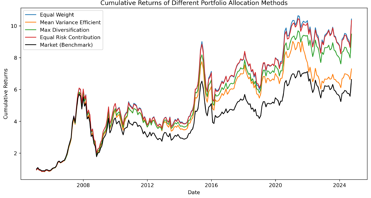
Cumulative returns of equal weight, mean-variance efficient, maximum diversification, and equal risk contribution allocations against the market, with equal weight and equal risk contribution on top and the mean-variance optimizer lagging

Equal weight and equal risk contribution finish at the top. The mean-variance efficient portfolio, the one that is theoretically optimal, actually lags them, because the estimation error in its inputs costs more than its cleverness earns. In Shi's stylized comparison the methods are identical when factors share Sharpe ratios and correlations, and the optimizer only pulls ahead in the fully general case, on paper, at Sharpe 0.670 versus equal weight's 0.504, which is precisely the case where the input sensitivity bites hardest in live trading. This is the old article "Collinearity in Parameter Sweeps: Plateaus, Not Peaks" applied to portfolios instead of parameter grids. There, the lesson was to trust a wide plateau of stable performance over a razor-thin peak that only exists because two parameters move together. Here, equal weight is the plateau: no inputs to estimate, nothing to overfit, robust by construction. Factor timing and mean-variance optimization are the peak: gorgeous at the estimated optimum, and standing on air the moment your estimates are off.

None of this says timing is impossible. It says the honest baseline is brutal. Before you deploy any timing signal, you owe it a comparison against equal weight with a real out-of-sample window and Newey-West standard errors, and most signals will not clear the bar. The edge that survives is narrow, it lives in the big common components rather than individual factors, it is timed by valuation rather than momentum or sentiment, and it is small enough that transaction costs can erase it. Sell the plateau, not the peak.

KEY POINTS

In Chuan Shi's Chinese study (2000 to 2020, top-1000 universe, seven long-leg factors), valuation, momentum, volatility, and sentiment timing all failed to beat an equal-weighted portfolio at every horizon, none reaching a t-statistic of 2.
The equal-weight benchmark itself was real, earning 0.27% a month over the market with a Newey-West t-statistic of 3.98. The timing overlays added nothing to it.
Valuation timing weights a factor by where its own value spread sits in its historical range, comparing each factor only to itself, never across factors.
Inverse-volatility weighting is undercut by common volatility: factor vols carry an average pairwise correlation of 0.65 across four style factors and 0.55 across 92 factors, so tilting toward the calmer factor is mostly noise.
Theory says timing should be huge: the mean-variance-efficient SDF loadings are inverse conditional covariance times conditional expected returns, and moving from static investing to full timing lifted the average SDF variance from 1.67 to 2.96, nearly doubling the Hansen-Jagannathan Sharpe ceiling.
The predictability is concentrated: the first principal component of fifty anomalies explains 25.8% of variance, and only the dominant components (PC1, PC4) show tradeable out-of-sample R-squared (4.82% and 3.52%). The obscure components are noise.
Timing the big common components by valuation earns a positive out-of-sample information ratio (0.60) while naive market timing earns minus 0.64. Timing works where the naive practitioner is not looking.
Equal weight and equal risk contribution beat the mean-variance optimizer in live trading because the optimizer's input-estimation error costs more than its cleverness earns. Prefer the robust plateau over the fragile peak.

References

- Factor Timing (Haddad, Kozak, and Santosh, 2020)
- Implications of Security Market Data for Models of Dynamic Economies (Hansen and Jagannathan, 1991)
- Macroeconomic Perceptions, Financial Constraints, and Anomalies (He, Su, and Yu, 2024)
- One Vol to Rule Them All: Common Volatility Dynamics in Factor Returns (Kapadia, Linn, and Paye, 2024)
- Factor Timing and Factor Allocation (Shi, 2024)
A note on AI. The ideas, research, analysis, and conclusions in this article are my own. I use AI tools to help with editing and wordsmithing, because English is not my first language, and I am not shy about that. AI-generated ideas and AI-assisted writing are not the same thing: the first is empty slop from a generic prompt, the second is a tool for communicating years of real research more clearly. Judge the work by its substance, not by whether software helped polish the prose.