10. Cross-Sectional & Factor Investing July 9, 2026 10 min

10.8 Selection vs Diversification: Why |t|>3 Throws Away Alpha

The |t|>3 rule is right for testing one factor, wrong for building a portfolio. A book of 18,000 signals, 80% noise, beats the strict filter because diversification pays where selection does not.

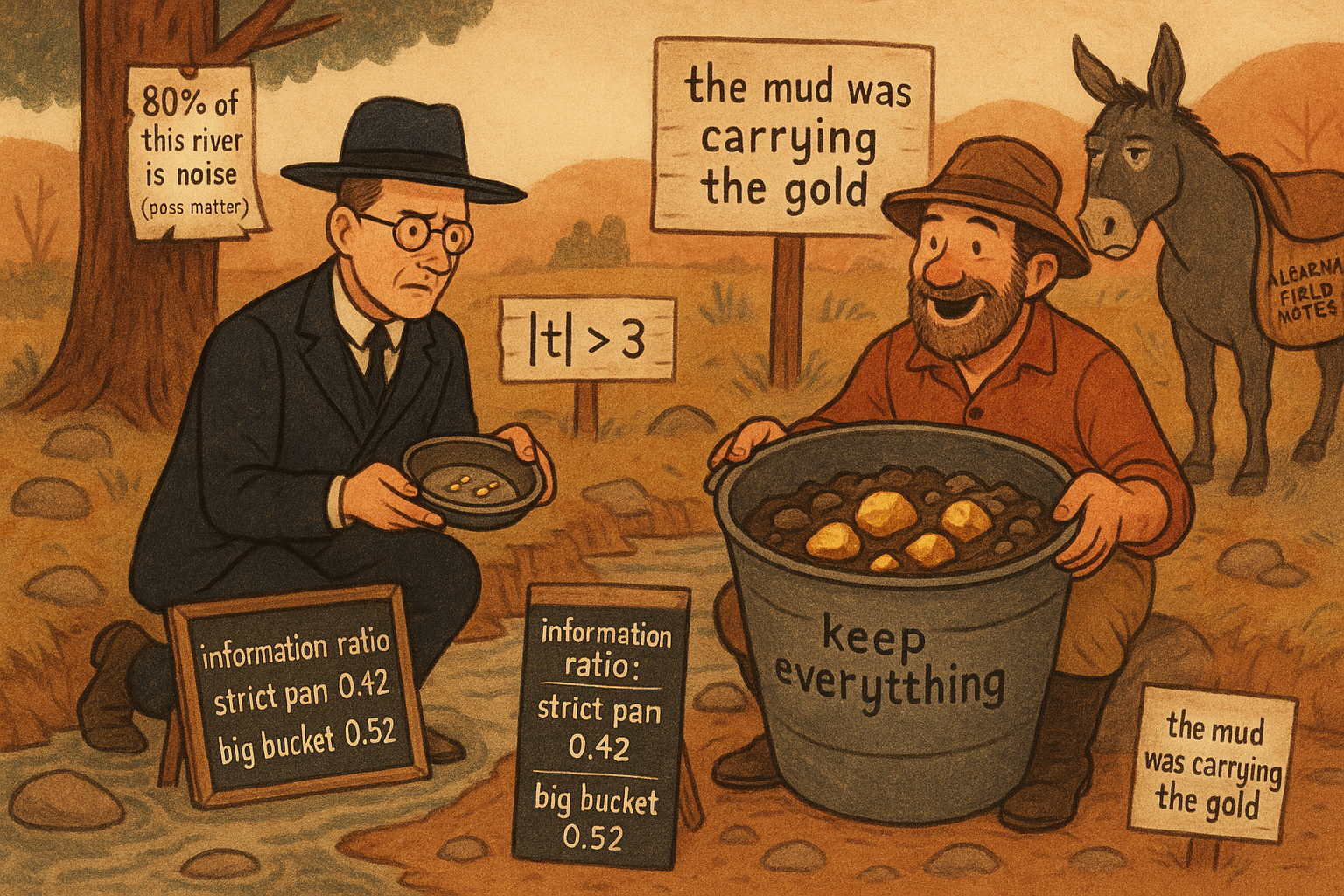
The factor-zoo reckoning handed the profession a clean rule: raise the bar. If a new predictor cannot clear a t-statistic of 3, treat it as noise. Harvey, Liu and Zhu built the case, Chordia, Goyal and Saretto pushed the cross-sectional hurdle to 3.4, and the field mostly nodded along. That rule is correct for the question it answers. The question is whether one specific signal is real. But almost nobody who quotes the rule is answering that question. They are building portfolios, and for portfolio construction the same rule quietly destroys performance.

Shingo Goto and Toru Yamada put a number on the damage. They rebuilt Yan and Zheng's data-mining machine, generated more than 18,000 fundamental-ratio signals, and found that roughly 80% of them are statistical nulls. Then they did the thing the inference crowd never bothers to do: they measured the out-of-sample information ratio of portfolios sorted by how strict the significance filter was. The strict bucket, the one that survives the |t|>3 hurdle, is the worst portfolio in the study. A portfolio that keeps every single signal, 80% garbage included, beats it. This article is about why, and about the exact point where the statistician's advice and the portfolio manager's payoff pull in opposite directions.

The old article "The Factor Zoo and the Multiple-Testing Reckoning" made the case for the high bar. This is the other side of that trade. And the old article "The Backtest Integrity Checklist" already flagged the discipline that decides who is right here: know what you are optimizing for before you pick a threshold.

The brackish environment: mostly noise, some real signal

Start with the raw material. Following Yan and Zheng, Goto and Yamada compute financial ratios across 213 Compustat accounting variables and 15 base denominators, sort stocks into deciles on each ratio every year, and form value-weighted long-short portfolios (top decile minus bottom decile). After requiring at least 120 consecutive months of returns, roughly 13,932 signal portfolios are eligible in an average year, peaking above 15,000 after 2005. That is an order of magnitude more predictors than there are stocks to predict, which is the defining feature of the modern factor problem.

How much of it is real? Storey's estimator says most of it is not. The fraction of null signals, the ones with a true alpha of exactly zero, comes in at 79.1% for CAPM-adjusted returns and 80.6% for FF6-adjusted returns. The picture below shows why that estimate is credible: the empirical distribution of p-values hugs the uniform 45-degree line for thresholds above 50%, exactly what pure noise produces, but piles up an obvious excess mass near zero.

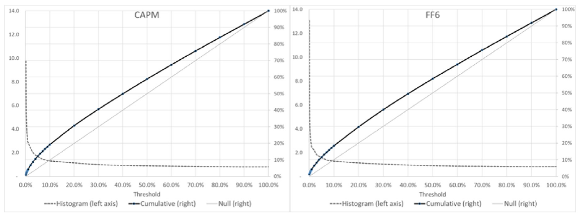
Empirical distribution of in-sample p-values for CAPM and FF6 alphas, showing a spike of small p-values against a mostly uniform bulk

The estimator reads that right tail. If almost every p-value above some cutoff belongs to a null signal, count them and scale up.

$$ \hat{\pi}_0(\lambda) = \frac{\#\{\, p_i > \lambda \,\}}{(1-\lambda)\, m} $$

Here m is the total number of signals, p-sub-i is the p-value of signal i, and lambda is a cutoff pushed toward one where non-null signals rarely survive. The count of p-values above lambda, divided by the number a uniform distribution would put there, estimates the null fraction pi-zero. Work it at lambda equal to 0.5: if a genuinely null world would scatter half its p-values above 0.5, and you observe about 40% of your 13,932 signals sitting up there, then pi-zero is roughly 0.40 divided by 0.50, near 0.80. Goto and Yamada minimize this across several lambdas and average across years to stay conservative, and still land at 79 to 81% null.

That leaves 19 to 21% non-null, about 2,700 to 2,900 real signals a year. Real, but pathetic on their own. The paper's maximum-likelihood fit puts the average non-null signal at a t-ratio of 1.62, which corresponds to a p-value near 10.5%. The typical true signal would fail |t|>3 by a mile. This is the brackish water in the paper's title: weak fresh signal dissolved in an ocean of salt, impossible to separate cleanly one drop at a time.

Two ways to count the false discoveries

Before measuring portfolios, measure the contamination. The false discovery proportion is the share of your "significant" signals that are actually null. Two estimators bracket it.

$$ \widehat{\text{FDP}}(\tau) \;=\; \hat{\pi}_0 \cdot \frac{\tau}{\hat{F}_p(\tau)} \qquad\qquad \text{Easy FDP}(\tau) \;=\; \frac{\tau}{\hat{F}_p(\tau)} $$

Read the pieces. Tau is the p-value threshold you call significant. F-hat-p of tau is the fraction of all signals that actually clear tau. The ratio tau over F-hat-p of tau is Chen's Easy FDP, an upper bound that needs no estimate of the null fraction, since under pure noise you expect a fraction tau to clear by luck and you compare that against how many actually did. Multiply by the estimated null fraction pi-zero and you get Storey's sharper plug-in estimate.

Work the conventional 5% threshold on CAPM alphas. Only 12.1% of signals clear it, so F-hat-p of 0.05 is 0.121. Easy FDP is 0.05 divided by 0.121, which is 0.413. So up to 41% of everything you just blessed at the 5% level is spurious. Fold in the 79.1% null rate and Storey's estimate drops to 0.791 times 0.413, about 0.327, still a third false. Even at the stringent 0.1% threshold the bound sits near 8 to 10%. The inference lesson is real: to get false discoveries below 5% you genuinely need to go tighter than |t|>3. If your job is to certify a single factor, the high bar is not paranoia, it is arithmetic.

The metric that matters for a portfolio is the information ratio

Now switch jobs. A portfolio manager does not care whether signal number 8,412 is individually real. The manager cares about return per unit of risk on the combined book. The relevant object is the information ratio.

$$ \text{IR} \;=\; \frac{\hat{\alpha}}{\hat{\omega}} \sqrt{12} \qquad\qquad t \;=\; \frac{\hat{\alpha}}{\hat{\omega}} \sqrt{T} $$

Alpha-hat is the portfolio's monthly benchmark-adjusted return, omega-hat is its residual risk, the standard deviation of what the benchmark cannot explain. Their ratio is the monthly information ratio, and multiplying by the square root of 12 annualizes it. The t-statistic is the same ratio scaled by the square root of the number of months, so a higher information ratio and a stronger t-stat are the same statement.

This is where strict selection destroys itself. Tightening the filter raises alpha per signal but shrinks the number of signals, and fewer signals means less diversification and higher residual risk. The residual risk climbs faster than the alpha. Take the CAPM numbers straight from the study. The strict p-less-than-0.1% bucket earns a monthly alpha of 0.268% on residual risk of 2.195%, so its information ratio is 0.268 divided by 2.195, times the square root of 12, which is 0.42. The loose p-less-than-6% bucket earns a smaller alpha of 0.191% but on residual risk of only 1.272%, giving 0.191 divided by 1.272, times root 12, which is 0.52. Lower alpha, higher information ratio. The strict bucket won the alpha contest and lost the only contest that pays.

The information ratio peaks where the statistician tells you to stop

Plot the information ratio against the significance threshold and the whole argument lands in one line.

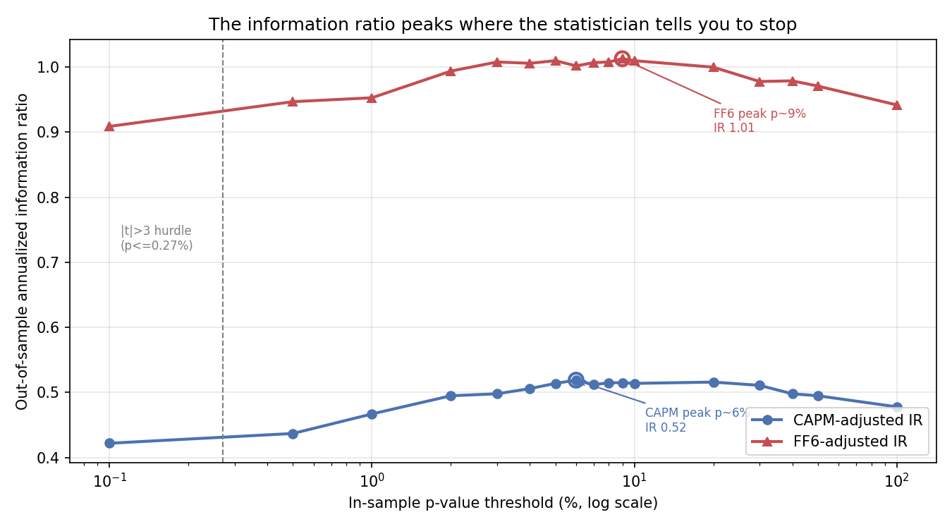
Out-of-sample annualized information ratio by in-sample p-value threshold for CAPM and FF6, peaking near 6 to 9 percent and lowest at the strict bucket

The peaks sit nowhere near the inference hurdle. For CAPM the best bucket is p-less-than-6%, holding around 1,900 signals at roughly 35% false discovery proportion, with an information ratio of 0.52 and a t-ratio of 3.29. For FF6 the peak is p-less-than-9%, information ratio 1.01, t-ratio 6.40. The strict p-less-than-0.1% bucket, the one that passes |t|>3, is the low point of both curves at 0.42 and 0.91. Harvey, Liu and Zhu recommend p-less-than-0.27%, Chordia and coauthors p-less-than-0.07%. Both sit to the left of the dashed line, in the exact region where the portfolio does worst.

Push it to the absurd end and the result holds. The bucket that keeps every signal, p-less-than-100%, roughly 80% of it null by construction, still beats the strict bucket: 0.48 versus 0.42 for CAPM, 0.94 versus 0.91 for FF6. Feeding a portfolio 80% pure noise beat the disciplined filter that the profession spent a decade defending. That is not a rounding error, it is the thesis.

Diversification, formalized: the Dybvig-Ross spanning test

"Beats" needs a test, not a Sharpe-ratio eyeball. Goto and Yamada use the classical spanning regression from Dybvig and Ross: to ask whether portfolio A adds anything a mean-variance investor wants beyond an existing portfolio B, regress A's returns on B's and look at the intercept.

$$ r_{A,t} \;=\; a \;+\; b\, r_{B,t} \;+\; \varepsilon_t $$

r-A-t and r-B-t are the excess returns of the two portfolios, b is A's beta to B, and epsilon is the leftover. The intercept a is the whole point. A positive, significant a means A delivers return that B cannot span, so adding A improves the frontier. A negative a means A is a drag. Set B to the strict p-less-than-0.1% benchmark and let A run through the looser buckets.

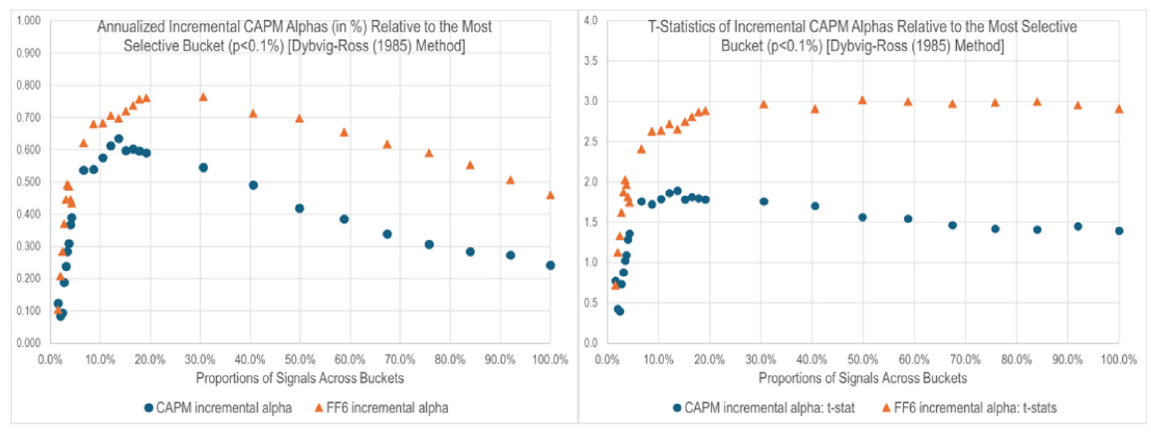
Incremental Dybvig-Ross alphas and t-statistics of each bucket over the strict benchmark, plotted against the proportion of signals included

The intercepts are positive almost everywhere. For FF6-adjusted returns every bucket above 3% delivers a positive, statistically significant incremental alpha, the largest at p-less-than-20% with 0.765% per year and a t-stat of 2.97, and the highest t-stat of 3.02 at p-less-than-40%. For CAPM the gains are more modest but still positive across a broad band, topping out at 0.635% per year at p-less-than-6%. Diversifying away from the strict bucket does not just look better, it spans the strict bucket and adds a frontier gain on top. The weak and null signals the inference rule told you to discard were carrying diversification you paid to throw away.

Why noise does not hurt: equal weighting is shrinkage in disguise

The mechanism is not mystical. A null signal has zero expected alpha by definition, so averaging it into an equal-weighted book does not drag the mean return down. What it does is dilute idiosyncratic estimation error. Every signal portfolio carries its own noise; average thousands of them and that noise partially cancels while any faint common alpha survives. Equal weighting across 14,000 signal portfolios is a brute-force version of the 1/N rule that Ledoit and Wolf and DeMiguel and coauthors show is hard to beat, and it behaves like implicit shrinkage and model averaging. It is the same instinct behind combining many weak indicators rather than betting the book on the single strongest one.

Strict selection does the opposite. Keeping only the handful of most-significant signals maximizes in-sample alpha and maximizes prediction-error variance at the same time. Weights get concentrated and unstable, residual risk balloons, and the information ratio collapses, which is exactly the curve you saw. There is even a harder version of the claim in the statistics literature the paper leans on: Bishop showed that deliberately injecting noise into training is equivalent to Tikhonov regularization. Under the right conditions, noise is not just harmless, it disciplines the fit.

Where this connects, and where it does not

Read this next to the old article "The Factor Zoo and the Multiple-Testing Reckoning" and the tension resolves. That reckoning is right that the tightest bar kills false factors. Goto and Yamada measure what else the tightest bar kills: the diversifying, individually-weak signals that carry portfolio performance. Same evidence, opposite prescription, because the objective changed from inference to construction. The old article "The Backtest Integrity Checklist" already made this the first question to ask, and this paper is the cleanest case for why. Pick your threshold to match your goal, not your journal.

Two honest caveats keep this from becoming a license to hoard noise. First, the portfolios are value-weighted on purpose, which strips out the microcap inflation that makes equal-weighted anomaly results look better than they trade. Second, the edge decayed. FF6 alphas in the strict bucket fell from 0.66% per month before 2003 to 0.19% after, a drop of roughly 70%, and Storey's diagnostics confirm it was not driven by more false discoveries but by genuine market efficiency and transaction costs eating the alpha. Diversification across signals still helps contain those costs through offsetting trades, but the free lunch shrank. The durable lesson is not "keep everything forever." It is that statistical significance and economic usefulness are different quantities, and a rule tuned for one will misprice the other.

KEY POINTS

The |t|>3 hurdle from the factor-zoo literature answers an inference question, whether one signal is real. It is the wrong tool for portfolio construction, where the payoff is return per unit of risk on the combined book.
Data-mining more than 18,000 fundamental signals, Goto and Yamada estimate roughly 80% are statistical nulls (Storey pi-zero of 79 to 81%), and the average real signal has a t-ratio near 1.62, far below any strict hurdle.
The out-of-sample information ratio peaks at loose thresholds, p near 6% for CAPM (IR 0.52) and 9% for FF6 (IR 1.01), while the strict p-less-than-0.1% bucket is the worst performer at 0.42 and 0.91.
A portfolio holding every signal, about 80% of it null, still beats the strict bucket, because tightening selection raises alpha per signal but raises residual risk faster, sinking the information ratio.
The Dybvig-Ross spanning test confirms it: looser buckets deliver positive, significant incremental alpha over the strict benchmark, up to 0.77% per year for FF6, so the discarded weak signals were carrying diversification.
Equal weighting across thousands of signals acts as implicit shrinkage and model averaging, diluting estimation noise while faint common alpha survives, which is why adding null signals does not hurt and can help.
Caveats: results are value-weighted to avoid microcap inflation, and FF6 alphas decayed roughly 70% after 2003 from market efficiency and costs, not from more false discoveries. Match the threshold to the objective.

References

- Fundamental Analysis and the Cross-Section of Stock Returns: A Data-Mining Approach (Yan and Zheng, 2017)
- ...And the Cross-Section of Expected Returns (Harvey, Liu, and Zhu, 2016)
- Anomalies and False Rejections (Chordia, Goyal, and Saretto, 2020)
- A Direct Approach to False Discovery Rates (Storey, 2002)
- Most Claimed Statistical Findings in Cross-Sectional Return Predictability Are Likely True (Chen, 2025)
- The Analytics of Performance Measurement Using a Security Market Line (Dybvig and Ross, 1985)
- Choosing Factors (Fama and French, 2018)
- Optimal Versus Naive Diversification: How Inefficient Is the 1/N Portfolio Strategy? (DeMiguel, Garlappi, and Uppal, 2009)
- Selection Versus Diversification in Noisy Alpha Environments (Goto and Yamada, 2026)
A note on AI. The ideas, research, analysis, and conclusions in this article are my own. I use AI tools to help with editing and wordsmithing, because English is not my first language, and I am not shy about that. AI-generated ideas and AI-assisted writing are not the same thing: the first is empty slop from a generic prompt, the second is a tool for communicating years of real research more clearly. Judge the work by its substance, not by whether software helped polish the prose.