4.78 Good vs Bad COVOL in Crypto: A Common-Volatility Tilt

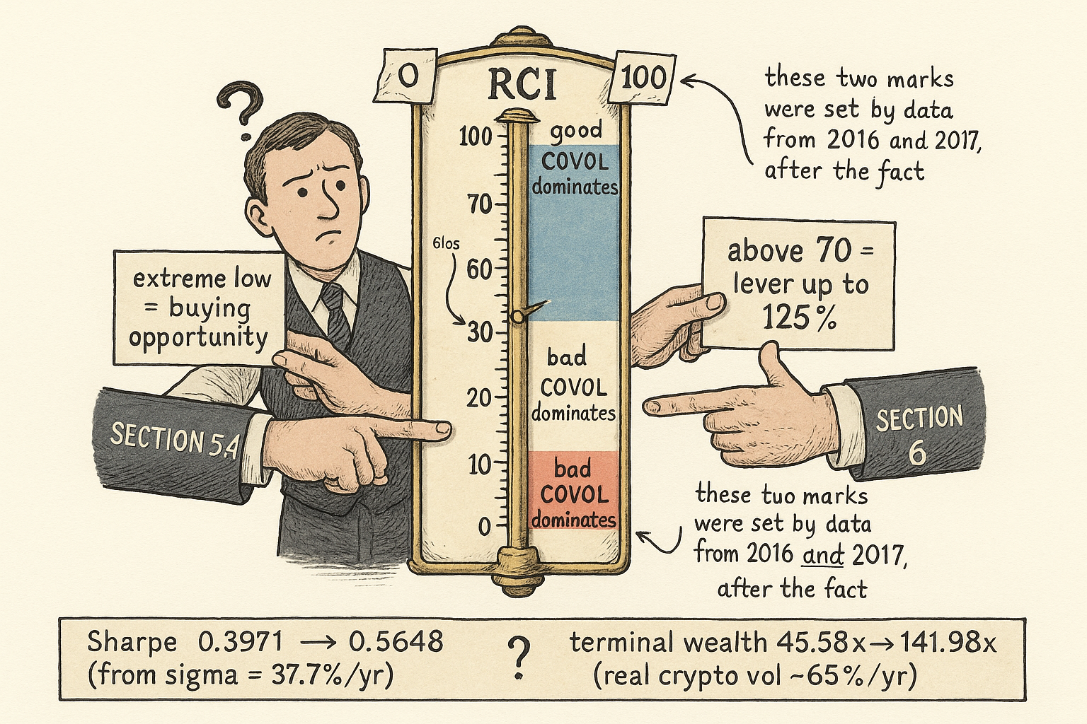
Pham, Han, Nguyen, Pham and Do build one index and then trade it backwards. In Section 5.4 they write that an RCI near zero marks "widespread panic selling and a potentially buying opportunity," and that exuberance at the top "can indicate a market peak and a potential selling opportunity." Nine pages later, in Section 6, they lever the portfolio up to 125% when the same index rises above 70 and cut it to 75% when it falls below 30. Contrarian in the diagnosis, momentum in the backtest, same number on both sides. The momentum version is the one that produced the headline, so the headline is the version that was not the paper's own stated reading of its own index.

That is worth sitting with before we get to the numbers, because the index itself is a genuinely good idea. Engle and Campos-Martins showed that if you fit a GARCH model to each asset separately, the leftover squared residuals still move together across assets. They named the latent factor driving that co-movement COVOL, and it measures something no news index captures: the days on which everything surprised at once. This paper applies it to 25 cryptocurrencies from January 2015 to April 2024, splits it by the sign of returns, and turns the split into a tradable tilt. The construction is clean. The evaluation is not.

One latent factor that rescales everybody's variance

Start with what COVOL actually is, because the word "volatility" is doing two jobs here. Each coin gets an AR(1) return equation with a first-principal-component factor and GARCH(1,1) errors, which strips out that coin's own predictable variance. What remains is the standardized residual, which by construction has unit variance. COVOL is a common multiplier on the variance of that residual.

$$ e_{i,t} = \sqrt{g(s_i\, x_t^{\sigma})}\; \epsilon_{i,t}, \qquad g(s_i\, x_t^{\sigma}) = s_i\,(x_t^{\sigma} - 1) + 1 $$

Read the second piece first. The latent factor x has mean one by construction, so on an average day the bracket is zero and g equals one, leaving the residual at its nominal unit variance. On a common-shock day x jumps above one, and each coin's variance gets multiplied by g, where the loading s decides how much of the shock that coin absorbs. Coins with a high s are the ones that blow up when the whole sector blows up.

Worked example with the paper's own numbers. Bitcoin's bad-COVOL loading is 0.2430, and the largest bad COVOL in the sample is 98.4933 on 3 April 2017. So g equals 0.2430 times 97.4933 plus 1, which is 24.69. Variance multiplied by 24.69 means volatility multiplied by the square root, 4.97. Bitcoin's return distribution that day was five times as wide as on a normal day, and that is on top of whatever its own GARCH process already knew. Run the same arithmetic on 12 March 2020, where bad COVOL was 43.5893: g is 11.35, so the volatility multiplier is 3.37. Toncoin, with a loading of 0.1123, gets 11.95 and 3.46 on the April 2017 date, so a coin with less than half Bitcoin's loading still absorbs a third more than Bitcoin did in March 2020. The loading compresses the extremes but does not remove them.

The test for whether a common factor exists at all is an equicorrelation test on the squared residuals, and it is worth checking because it is the gate everything else passes through.

$$ T_{e^2} \;=\; \hat{\rho}_{e^2}\,\sqrt{\frac{T\,N\,(N-1)}{2}} $$

The statistic is the average pairwise correlation of the squared standardized residuals, scaled by the square root of the number of pair-days in the panel, and it is standard normal under the null of no common volatility. The paper prints the statistic in an expanded form; collapsing it gives this, and the collapse is where the check lives. They report a correlation of 0.043 and a statistic of 20.67 with 25 coins. Invert it: the implied number of full-panel-equivalent days is 20.67 squared divided by 0.043 squared divided by 300, which is 770. Their goodness-of-fit pass, after the common factor is removed, reports a correlation of 0.0013 and a statistic of 0.635, and the same inversion gives 795. Those two agree, which confirms both statistics come from the same scale and that the printed equation is the right one. The p-value they quote for 0.635, namely 0.2627, is exactly one minus the standard normal CDF at 0.635, so that reconciles too.

The gap worth naming: the panel runs 3,361 days for Bitcoin, and 770 full-panel-equivalent days is what you get when most of the 25 coins only exist for the back half of the sample. Solana contributes 1,367 days, Toncoin 490, Mantle 267. The common factor in the early years is estimated off a handful of coins, and the RCI's historical extremes all sit in exactly those early years.

Splitting the factor by truncating returns, which breaks the error assumption

The good and bad decomposition is mechanically simple. Take each coin's return series, keep the positive days and set the rest to zero to get one series, then keep the negative days and set the rest to zero to get the other.

$$ \tilde{r}_{i,t}^{+} = \begin{cases} \tilde{r}_{i,t} & \tilde{r}_{i,t} > 0\\[2pt] 0 & \text{otherwise} \end{cases} \qquad \tilde{r}_{i,t}^{-} = \begin{cases} \tilde{r}_{i,t} & \tilde{r}_{i,t} \leq 0\\[2pt] 0 & \text{otherwise} \end{cases} $$

Then run the whole AR(1)-GARCH-plus-COVOL machine on each half separately. Good COVOL is the common variance factor of the positive-only series, bad COVOL the same for the negative-only series.

The problem is what that truncation does to the series being modelled. Roughly half the observations are now exactly zero. Take a coin with 3,361 days and a return that is positive on about 52% of them: the positive-only series has about 1,600 real numbers and 1,760 exact zeros. A GARCH(1,1) fit to that produces standardized residuals with a point mass at a single value, which cannot be the independent standard normal that the COVOL specification assumes for epsilon. The estimator does not know it is being fed a censored series. Patton and Sheppard, whom the paper cites as precedent, avoided this by building signed realized semivariances out of intraday returns, so every day carries both an up and a down measure and nothing gets zeroed. Splitting daily closes does not have that escape. The good and bad COVOL estimates are therefore point estimates under a violated distributional assumption, and the paper never reports the fit diagnostics for the split models the way it does for the pooled one.

Separately, the transcription is loose in places that matter for a reader trying to reimplement. The GARCH variance equation carries time subscripts on its parameters, which would make them non-identified; beta serves as both the factor loading in the mean equation and the persistence term in the variance equation; Section 5.3.3 points at "Equation (10)" when it means Equation (13); Figure 3's discussion cites "Table 10" when it means Table 5; Table 1's note dates the sample from January 2006 when the data section says January 2015; and Bitcoin's minimum excess return prints as 21.59 without the minus sign. None of that changes a result. All of it means you should check the arithmetic yourself rather than lift numbers.

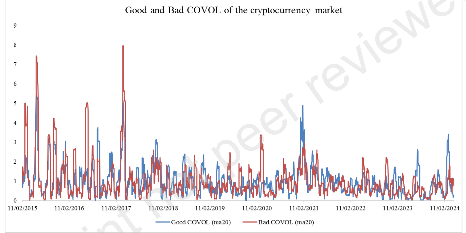
Two features of that picture carry the paper. Bad COVOL spikes harder, topping 8 in early 2017 against good COVOL's 5. Good COVOL happens more often: the authors count 1,754 days where good exceeded bad against 1,588 the other way, so 52.5% of days lean bullish. Frequent mild optimism against rare violent fear is the same asymmetry equity researchers have documented for decades, and finding it again in crypto is a reasonable contribution on its own. The amplitude also collapses after 2018 in both series, which tells you the whole sector's common-shock intensity fell by more than half once the panel filled out with real coins. Any threshold calibrated on the 2015 to 2017 amplitude describes a market that stopped existing.

The RCI, and why you could not have computed it at the time

The index is the difference between the two factors, smoothed and rescaled.

$$ d_t = \hat{\chi}_t^{\sigma,+} - \hat{\chi}_t^{\sigma,-}, \qquad dma_{20,t} = \frac{1}{20}\sum_{k=0}^{19} d_{t-k}, \qquad RCI_t = 100 \times \frac{dma_{20,t} - \min(dma_{20})}{\max(dma_{20}) - \min(dma_{20})} $$

Subtract bad from good, average the last 20 days of that difference, then map the result onto 0 to 100 by its distance between the minimum and the maximum. Worked example: suppose the 20-day average difference today is +1.2, the sample minimum is -4.0 and the sample maximum is +3.0. Then RCI equals 100 times (1.2 plus 4.0) divided by 7.0, which is 74.3, and the strategy levers up. Now suppose a later crash drops the minimum to -6.0. The identical +1.2 reading becomes 100 times 7.2 divided by 9.0, which is 80, and if the crash instead pushed the maximum to +5.0 the same reading becomes 100 times 5.2 divided by 11.0, which is 47.3, and the strategy sits flat rather than levering. One reading, three answers, decided by data that had not happened yet.

That is the defect. The min and max in Equation (12) are taken over the whole sample, so the 30 and 70 thresholds are not observable in real time. A trader standing in June 2018 does not know what the 2021 extremes will be.

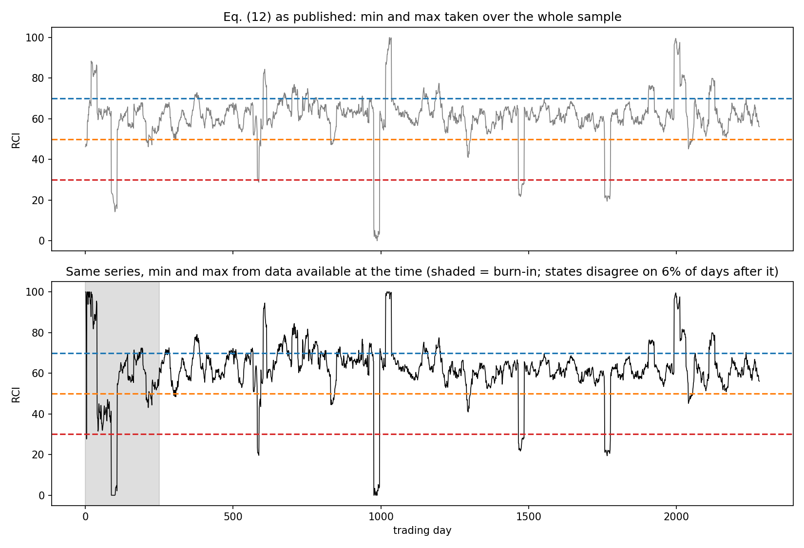
I simulated two spiky mean-one factors, differenced them, and computed the index both ways to see how much the choice matters. With full-sample scaling the index sits above 70 on 10.2% of days after burn-in; with expanding-window scaling, the only version you could trade, it sits above 70 on 15.9%. The three-state signal disagrees on 6% of days. A strategy that takes leverage 56% more often than the published version is a different strategy.

Now the fair part, because the size of this particular leak is smaller than the principle suggests. The extremes that set the denominator for this sample land early: good COVOL peaks in September 2016 at 58.9349 and bad COVOL peaks in April 2017 at 98.4933. The portfolio simulation starts in March 2017. So the full-sample range is essentially pinned within two months of the simulation's first trade, and only about one month of the 86 is contaminated. The leak is structural rather than fatal here. Had the extremes arrived in 2021 instead, every signal before them would have been fiction, and nothing in the method tells you in advance which sample you are in. Rebuild it with an expanding or rolling range and report both. The old article "Percentile-Rank Momentum With Hysteresis: Low-Churn Signals" makes the same point from the other direction: rank-based signals need their reference window fixed to information available at decision time, and they need hysteresis so a threshold crossing does not flip the book on noise.

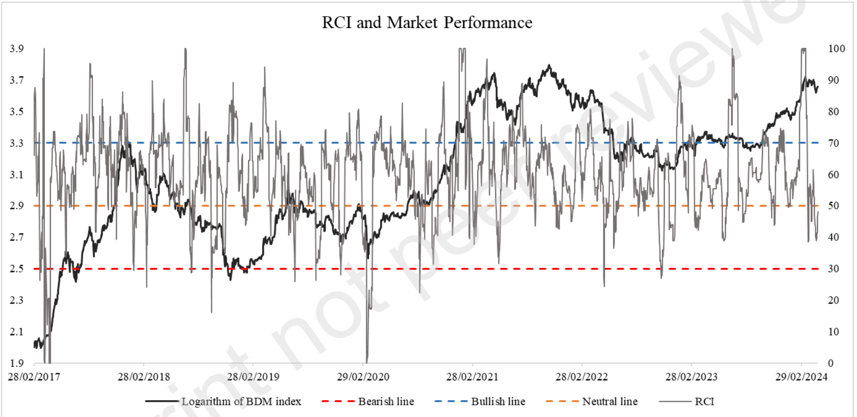
Look at that chart with the direction question in mind. The RCI is a difference of two variance factors, and neither factor knows the sign of the market's return. Good COVOL is high when positive returns were commonly large in magnitude, which happens in melt-ups and also in violent bear-market rallies. The index reads direction only because in crypto, large synchronized up-moves cluster inside bull markets. That is an empirical regularity, not an identity, and it is the reason the paper could argue itself into both a contrarian and a momentum reading without noticing. The old article "Regime-Switching That Works, Factors That Don't (MS-GARCH)" found the same asymmetry: a second-moment model can label the regime you are in with real skill while telling you close to nothing about the sign of the next return.

The tilt is smaller than the result it is credited with

Here is what the strategy actually does. Above 70, hold 125% of the crypto index. Below 30, hold 75%. In between, hold 100%. Borrow and lend at the one-year Treasury yield. The thresholds come from RSI convention, which the authors state openly, so at least they are not fitted.

Everything the tilt earns over buy-and-hold comes from the covariance between the weight and the return.

$$ R_t^{\text{RCI}} - R_t^{\text{B\&H}} = (w_t - 1)\,(r_t - r_f), \qquad \mathbb{E}\!\left[R^{\text{RCI}} - R^{\text{B\&H}}\right] = 0.25\left(p_{+}\,m_{+} - p_{-}\,m_{-}\right) $$

The weight deviates from one by 0.25 in either direction, so the monthly edge is 0.25 times the frequency of bullish months times their mean excess return, minus 0.25 times the frequency of bearish months times theirs. Worked example with the paper's means: RCI Momentum 1 averages 2.48% a month against 1.91% for buy-and-hold, a gap of 0.57%. Divide by 0.25 and the signal must deliver 2.28 percentage points a month of frequency-weighted spread. If the bullish and bearish states each occupy 20% of months, the conditional means must differ by 11.4 points a month. At 30% each, 7.6 points. Crypto monthly returns are wide enough that this is possible, and that is the entire bet: a ±25% exposure wobble pays only if the index separates monthly returns by high single digits at minimum.

Except the paper's own outperformance columns disagree about how large that spread was. The terminal wealth ratio, 141.98 against 45.58, is 3.115 over 86 months, which compounds to 1.33% a month of relative gain and by the same arithmetic demands 5.32 points a month of spread. The arithmetic means demand 2.28. The two are a factor of 2.3 apart.

Table 6 does not describe one return series

That inconsistency is worth running down, because the headline lives in this table.

$$ g \;\approx\; m - \tfrac{1}{2}\sigma^2, \qquad SR = \frac{(1+g)^{12} - 1 - r_f}{\sigma\sqrt{12}} $$

The geometric monthly return is the arithmetic mean less half the variance, and the annualized Sharpe compounds that geometric mean, subtracts the risk-free rate and divides by the annualized volatility. Run it on buy-and-hold: m is 1.91%, sigma is 10.89%, so g is 1.317%, compounding to 17.00% a year against an annualized volatility of 37.72%, and with a 1.8% Treasury yield the Sharpe is 0.403. Reported, 0.3971. Run it on RCI Momentum 1: g is 1.832%, annualizing to 24.35% against 39.42%, giving 0.572 against a reported 0.5648. The mean, standard deviation and Sharpe columns hang together.

The accumulated return column does not hang with them, on either reading. Read 45.58 as a percentage and buy-and-hold compounded at 0.438% a month for 86 months, which against an arithmetic mean of 1.91% implies a volatility drag of 1.47 points a month and therefore a monthly standard deviation of 17.2%, not the 10.89% printed beside it. Read 45.58 as a terminal wealth multiple and the geometric mean becomes 4.54% a month, which exceeds the arithmetic mean of 1.91%, and a geometric mean can never exceed an arithmetic one. Neither reading survives.

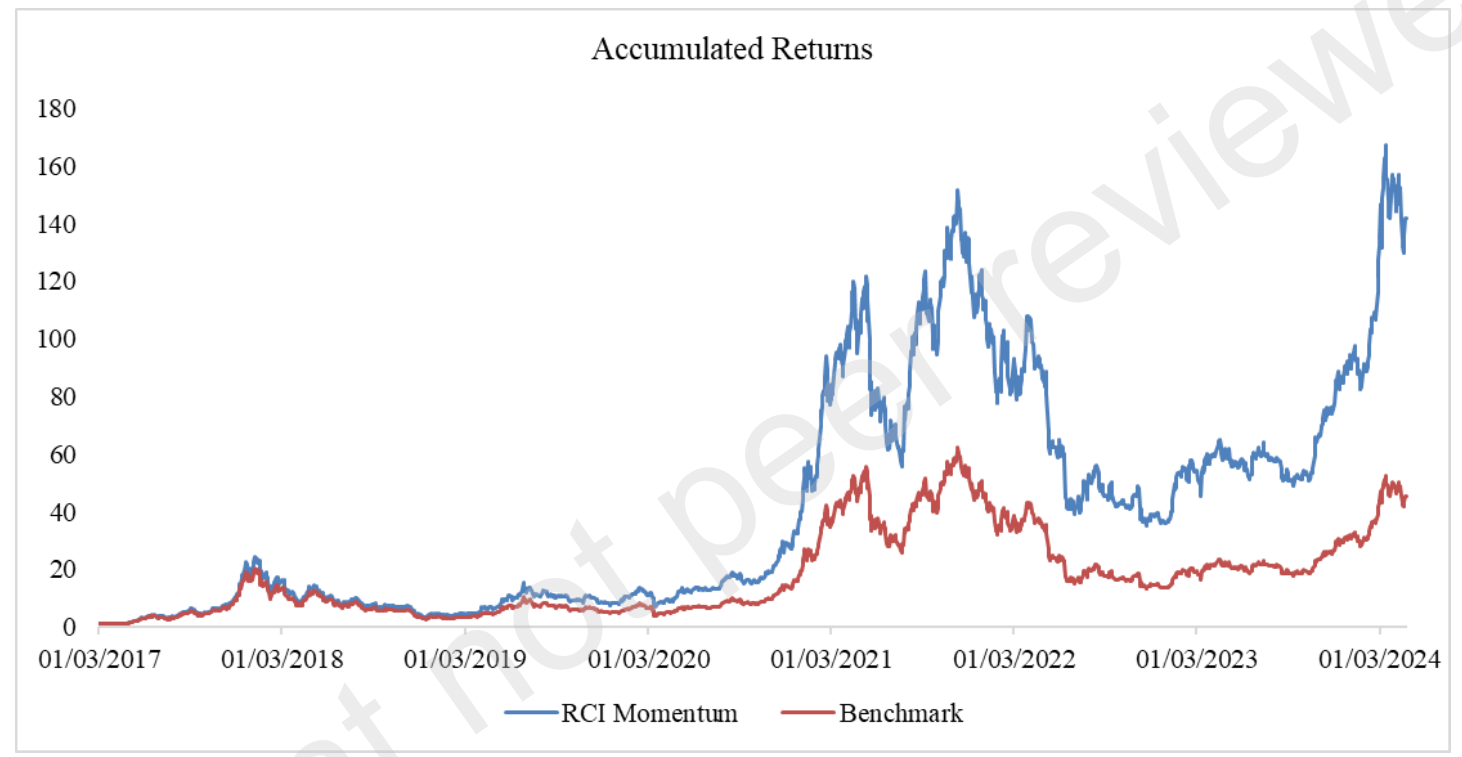
The figures settle which column describes reality. Figure 5 puts the logarithm of the BDM index at about 1.95 in February 2017 and about 3.65 in early 2024. Base-ten logs on an index based near 100 give a rise from roughly 89 to roughly 4,470, a factor near 50, which matches the market: Bitcoin went from about 1,180 dollars to about 63,000 dollars over that window, a factor of 53. So 45.58 is a wealth multiple and buy-and-hold made about 4,458%, not 45.58%. And then the printed volatility of 10.89% a month, or 37.7% a year, belongs to no crypto index over 2017 to 2024; realized Bitcoin volatility over that period runs closer to 60% or 70% a year.

Keep the source form, because guessing at a correction is worse than reporting the conflict. Stated plainly: the risk-adjusted numbers everyone will quote, 0.5648 against 0.3971, were computed from a mean and a standard deviation that cannot have come from the series plotted in Figure 6. The relative result, 3.1 times the terminal wealth from a ±25% tilt, is the claim that matches the chart. Both cannot be right, and the paper does not reconcile them. This is also gross of costs. The tilt trades a broad index at monthly frequency, so turnover is low and the cost drag is small, but the leveraged leg borrows at the Treasury yield rather than a crypto broker's rate, and in 2021 those differed by more than a thousand basis points.

The macro drivers explain one percent

The last section regresses daily COVOL on a risk-aversion index, the S&P 500 return, the dollar index, the ten-year-minus-two-year term spread and the two-year yield. The signs are sensible: the dollar comes in negative, the term spread and the short yield positive. The adjusted R-squared is 0.0105.

One percent of the variation in COVOL, across 2,219 days. The paper calls these "crucial macroeconomic and sector-specific drivers." Significance at that sample size costs almost nothing, and two of the stars do not survive their own standard errors: the dollar coefficient of -0.05 with a standard error of 0.03 is a t of -1.67, which is the 10% level and not the 5% level it is marked at, and the monthly crypto-price-uncertainty coefficient of 0.017 with a standard error of 0.09 is a t of 0.19, marked significant at 10%. That last one is almost certainly a typo for 0.009, which gives a t of 1.89 and does clear 10%, but the table as printed does not support its own asterisk. The monthly specification reaches an adjusted R-squared of 0.1657 on 102 observations, which is more respectable and also 102 observations.

The validation tests are the strongest empirical section and get the least attention. Squared COVOL predicts the broad index's realized volatility with a coefficient of 0.42 and survives at 0.38 in the full model with global policy uncertainty, VIX changes and geopolitical risk alongside it, where policy uncertainty loses its significance. Squared COVOL also raises the average pairwise correlation among the 25 coins with a coefficient of 0.02: a move in monthly squared COVOL from 1 to 10 lifts average pairwise correlation by 0.18, which is the difference between a diversified crypto book and one position. That is the finding I would build on. It says nothing about direction and everything about when your diversification stops working.

KEY POINTS

• COVOL is one latent factor that multiplies every coin's post-GARCH residual variance, scaled per coin by a loading. Bitcoin's bad-COVOL loading of 0.2430 against the sample's worst bad COVOL of 98.4933 gives a variance multiplier of 24.69, so a volatility multiplier of 4.97. On 12 March 2020 the same arithmetic gives 3.37.
• The equicorrelation test reconciles twice. A correlation of 0.043 with a statistic of 20.67 and a post-fit correlation of 0.0013 with a statistic of 0.635 both imply about 780 full-panel-equivalent days out of a 3,361-day panel, which is what an unbalanced panel of late-listing coins produces. The quoted p-value of 0.2627 matches the normal CDF exactly.
• The good and bad split truncates daily returns to zero on half the days and then fits GARCH to the result. Standardized residuals from a series with a point mass at zero cannot be the independent standard normal the COVOL specification assumes. Patton and Sheppard dodged this with intraday semivariances; splitting daily closes has no such escape.
• Equation (12) rescales the index by the whole sample's minimum and maximum, so the 30 and 70 thresholds were unknowable in real time. In simulation the tradable expanding-window version sits above 70 on 15.9% of days against the published 10.2%. For this particular sample the extremes land in September 2016 and April 2017, just before a March 2017 start, so the leak is structural rather than decisive. Rebuild with a rolling range and report both.
• The RCI is a difference of two variance factors, so it carries no information about the sign of returns except through crypto's habit of clustering large synchronized up-moves inside bull markets. The paper reads it contrarian in Section 5.4 and momentum in Section 6, and only the momentum reading produced the headline.
• A ±25% exposure tilt earns the covariance between weight and return, nothing else. The 0.57% monthly gap over buy-and-hold requires 2.28 points a month of frequency-weighted conditional spread, or 11.4 points if the bullish and bearish states each occupy a fifth of months. The terminal wealth ratio of 3.115 demands 5.32 points instead, so the paper's two outperformance measures disagree by a factor of 2.3.
• Table 6's mean, standard deviation and Sharpe columns reconcile with each other: 1.91% and 10.89% monthly compound to 17.0% a year against 37.7% volatility and a Sharpe of 0.403 against the reported 0.3971. The accumulated return column reconciles with neither. As a percentage it implies 17.2% monthly volatility; as a wealth multiple it implies a geometric mean above the arithmetic mean, which is impossible. Figure 5's log scale and Bitcoin's 53-fold rise say it is a wealth multiple, which leaves the printed 37.7% annualized volatility describing no crypto index that existed. Source numbers kept as printed; the source appears wrong.
• Macro drivers explain 1.05% of daily COVOL variation across 2,219 days, with the dollar index starred at 5% on a t of -1.67 and crypto price uncertainty starred at 10% on a t of 0.19. Build instead on the validation result: squared COVOL moving from 1 to 10 lifts the average pairwise correlation across the 25 coins by 0.18, which is diversification failing on schedule.

References

• What are the events that shake our world? Measuring and hedging global COVOL - Engle & Campos-Martins (2023)
• Good Volatility, Bad Volatility: Signed Jumps and the Persistence of Volatility - Patton & Sheppard (2015)
• Good Volatility, Bad Volatility, and the Cross Section of Stock Returns - Bollerslev, Li & Zhao (2020)
• Asymmetric connectedness on the U.S. stock market: Bad and good volatility spillovers - Baruník, Kočenda & Vácha (2016)
• The cryptocurrency uncertainty index - Lucey, Vigne, Yarovaya & Wang (2022)
• The Time Variation in Risk Appetite and Uncertainty - Bekaert, Engstrom & Xu (2022)
• Measuring Geopolitical Risk - Caldara & Iacoviello (2022)
• Good versus Bad COVOL in Cryptocurrency Markets: A Measure of Asymmetric Common Volatility - Pham, Han, Nguyen, Pham & Do (ssrn-6038623)