9.43 Trend Quality Near Settlement: A Kalshi State Variable, Not Alpha
Kalshi trend quality (TQR) sorts pre-close contracts into a 19.6pp continuation gap, then dies out of sample: midquotes cut it to 1.9pp, AUC 0.448. A stand-down gauge, not alpha.
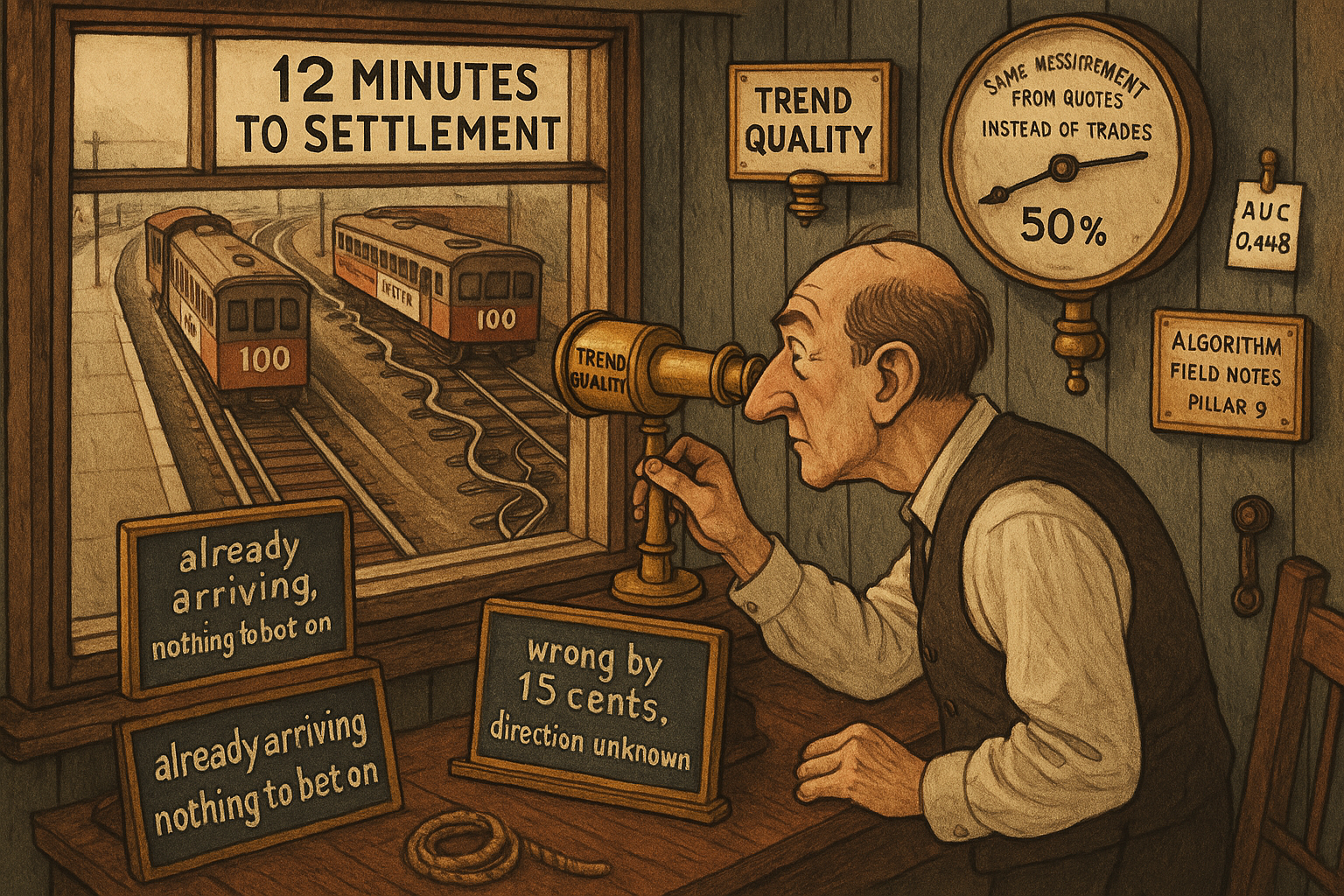
A 70.8% continuation rate looks like a trade. Greene sorts 4,061 Kalshi contracts by the quality of their price trend over the window from 30 to 12 minutes before close, and the top decile keeps moving in the trend's direction 70.8% of the time against 51.2% in the bottom decile. Ex-post forecast error falls from 14.75 cents to 6.07 cents across the same sort. Both gaps carry contract-level bootstrap p-values under 0.001. Then the same paper reports that the out-of-sample R-squared of the trend-quality signal is negative on every continuous target it tries, and that recomputing the whole exercise from quote midprices instead of last trades cuts the continuation gap from 19.6 points to 1.9 points with a p-value of 0.62. Both facts are in the paper. Only one of them made the abstract.
The statistic is called the Trend Quality Ratio, and the honest reading is that it describes a Kalshi market's state near settlement rather than predicting its next move. High trend quality marks a contract whose price has already worked out the answer. That is worth knowing. It is the opposite of a signal to trade, because you profit when a price is wrong, not when it is right. This sits next to the old article "Do Polymarket Prices Converge? Bias and Volatility Evidence," which measured the same convergence from the other side, and next to the old article "Percentile-Rank Momentum With Hysteresis: Low-Churn Signals," which treats a trend score as a state gate rather than an entry trigger.
The data deserves a note before any of the numbers. The panel holds 4,858,323 near-expiry snapshots across 29,590 tickers from 25 January to 12 March 2026, which sounds enormous. Greene discloses that a single BTC price-range series, KXBTC, contributes about 89% of those raw rows while making up 12% of tickers and 19% of the baseline contract windows. The analysis runs at contract level, so the skew does not weight the results, but "4.86 million snapshots" describes the disk, not the evidence. The evidence is 4,061 contracts with a non-zero trend, of which 1,094 resolved inside the sample.
The statistic, and the normalization that cancels itself
Fit a straight line to a contract's price over the pre-close window, with elapsed time running from 0 at 30 minutes remaining to 18 at 12 minutes remaining, and require at least 5 observations. Take the slope, divide by mean price to get a directionality index. Take the root mean squared residual, divide by mean price to get a normalized RMSE. Divide the first by the second.
$$ \text{DI} = \frac{\beta_1}{\bar{y}}, \qquad \text{nRMSE} = \frac{\sqrt{\frac{1}{n}\sum_{i=1}^{n} (y_i - \hat{y}_i)^2}}{\bar{y}}, \qquad \text{TQR} = \frac{\text{DI}}{\text{nRMSE}} = \frac{\beta_1}{\text{RMSE}} $$
Read it as drift per unit of noise. Beta-one is how many cents the fitted line climbs per minute; RMSE is how far the actual prints scatter around that line in cents. A contract that walks 9 cents higher in a tidy line scores high. A contract that ends 9 cents higher after thrashing around scores low.
Note the last equality, because the paper's own equations 2, 3 and 4 imply it and the paper never writes it down. Mean price appears in the numerator of the directionality index and in the numerator of the normalized RMSE, so it cancels exactly. Worked example: a contract averaging 40 cents, slope 0.50 cents per minute, residual RMSE 1.20 cents. The directionality index is 0.50 divided by 40, which is 0.0125 per minute. The normalized RMSE is 1.20 divided by 40, which is 0.030. The ratio is 0.0125 over 0.030, which is 0.4167. Now take the identical price path shifted up to an 80-cent mean: the directionality index halves to 0.00625, the normalized RMSE halves to 0.015, and the ratio is 0.4167 again. Straight to the point, beta-one over RMSE is 0.50 over 1.20, which is 0.4167.
Section 4.1 spends a paragraph arguing that dividing both pieces by mean price makes TQR "comparable across contracts with heterogeneous price levels." Nothing in the construction does that work. The ratio of a slope in cents per minute to a dispersion in cents is scale-free before you touch it, because both quantities scale linearly in the price. The two divisions by mean price are algebraic decoration.
The same paragraph calls TQR a "dimensionless" score. It is not. Cents per minute divided by cents leaves one over minutes. Our worked example scores 0.4167 per minute; measure elapsed time in seconds instead of minutes and the same price path scores 0.00694. Every decile cut point in the paper depends on the choice of clock. Greene fixes the window at 18 minutes and the unit at minutes for every contract, so the cross-sectional comparison inside this paper survives. The dimensional claim in the text does not, and anyone porting TQR to a 5-minute or 2-hour window has to refit the thresholds from scratch. I am keeping the source's form and flagging it rather than quietly redefining the statistic.
TQR is an effect size, not evidence
A reader who has fit a trend line before will ask why not use the t-statistic on the slope. The paper addresses this in prose and drops the algebra, which hides the interesting part.
$$ t_{\beta_1} = \frac{\beta_1}{s\,/\sqrt{S_{xx}}}, \qquad s = \text{RMSE}\sqrt{\frac{n}{n-2}}, \qquad S_{xx} = \sum_{i=1}^{n} (x_i - \bar{x})^2 $$ $$ \Longrightarrow \quad t_{\beta_1} = \text{TQR}\,\sqrt{S_{xx}\,\frac{n-2}{n}} $$
The OLS standard error uses the residual standard deviation s, which divides the squared residuals by n minus 2, while the paper's RMSE divides by n. Correct for that and the t-statistic is TQR multiplied by the square root of the regressor's total sum of squares, scaled by n minus 2 over n. Sum over the window observations; x is elapsed minutes.
Worked example with the dense case. Nineteen one-minute prints across the 18-minute window put x at 0 through 18, so the mean is 9 and the sum of squared deviations is 570. The factor 17 over 19 gives 510, whose square root is 22.58. Our TQR of 0.4167 corresponds to t equal to 9.41. Now the sparse case: the same TQR on the 5-point minimum, with prints at 0, 4.5, 9, 13.5 and 18 minutes elapsed, gives a sum of squared deviations of 202.5, a factor of 3 over 5, and t equal to 4.59. Same trend quality, half the statistical evidence.
That is the honest description of what a TQR sort does. It ranks contracts by effect size, the way a Cohen's d ranks group differences, and stays silent about how much data backs each estimate. Applying it to the bottom decile makes the point: mean TQR of 0.024 on 19 prints implies t equal to 0.54, which is no trend at all. The top decile's 0.574 implies t equal to 12.96. So the sort separates flat contracts from steep ones, and inside any one decile it pools a five-print guess with a nineteen-print measurement. Greene does carry window observations as a regression control, and that control lands at 0.065 with a standard error of 0.025 on forecast error, so sampling density is doing measurable work. The decile sorts do not control for it at all.
The continuation ladder, and the ties it is built on
Continuation asks whether the price observed closest to expiration sits on the trend's side of the price at 12 minutes remaining. Roughly 49% of non-zero-trend windows show exactly zero change over that stretch, which leaves the binary outcome undefined for half the sample. Greene handles this with a tie-adjusted score that scores a tie as half a win.
$$ \text{Cont}^{0.5} = (1-z)\,c \;+\; \tfrac{1}{2}z \qquad \Longleftrightarrow \qquad 2\,\text{Cont}^{0.5} - 1 = (1-z)\,(2c-1) $$
Here z is the share of windows with zero post-window change and c is the continuation rate among the windows that did move. The right-hand form is the one a trader wants, because 2c minus 1 is the directional edge on a coin-flip payoff and one minus z is the fraction of the time you get paid at all.
Check it against the paper's own table. The top decile reports c equal to 70.8% with z equal to 42.6%, so the edge is 0.574 times 0.416, which is 0.2388, and the tie-adjusted score is 61.94%. Greene reports 61.9%. The bottom decile reports 51.2% with z equal to 30.0%, giving 0.700 times 0.024, which is 0.0168, and a score of 50.8% against the paper's 50.9%. Decile 4 reports 57.2% with z equal to 64.3%, giving 52.6% on the nose. Table 1 and Table 2 reconcile to a tenth of a point.
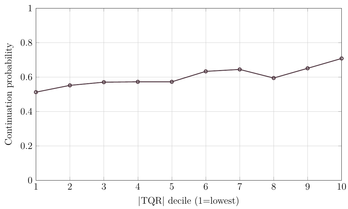
The ladder is the bull case, and it is not a clean ladder. Deciles 3 through 5 sit flat at 57%, decile 8 drops to 59.4% below deciles 6 and 7, and the whole rise is 19.6 points across a nine-step sort whose fitted slope is 1.8 points per decile. Two other things matter more than the wiggle. Continuation conditions on the post-window move being non-zero, which is a property of the outcome, so you cannot filter on it at entry. And continuation records only the sign of the move. Section 4.2 defines a magnitude-weighted version, the signed post-window change in cents, and no table in the paper reports it.
The error result reads backwards for a trader
Absolute forecast error is the gap between the price at 12 minutes remaining and the settlement value of 0 or 100 cents. Across the |TQR| sort it falls from 14.75 cents in the bottom decile to 6.07 cents in the top, an 8.68-cent improvement that Greene correctly reports as a 58.9% reduction. Then look at the path it takes to get there.
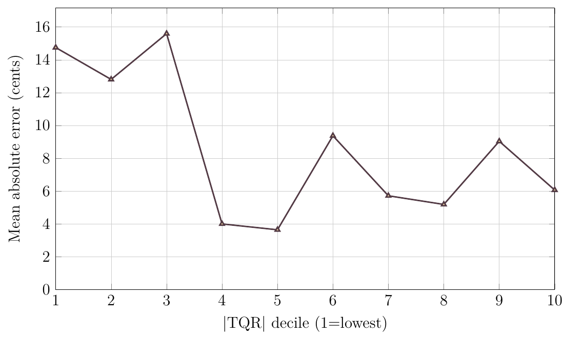
Deciles 4 and 5 post the lowest errors in the table at 4.00 and 3.64 cents, well below the top decile's 6.07. Decile 3 posts the highest at 15.60, above the bottom decile. The paper says this plainly, that the series "is not strictly monotone" and that individual decile means are noisy at a resolved sample of 1,094. Two further things are worth extracting.
First, the arithmetic. Average the ten decile error means without weights and you get 8.62 cents, while Table 4 reports an overall mean of 7.41. The gap has to come from unequal numbers of resolved markets per decile, which means the N column in Table 1 (407, then 406 nine times) describes the trend-quality deciles and not the error column that sits beside it. The resolved counts behind each decile mean are never printed. Under the midrange restriction this bites hard: 1,317 contracts pass the 20-to-80-cent filter, only 227 of them resolved, and the paper still prints ten decile error means with bootstrap intervals. That is roughly 23 resolved markets per decile carrying the headline 20.98-cent midrange result.
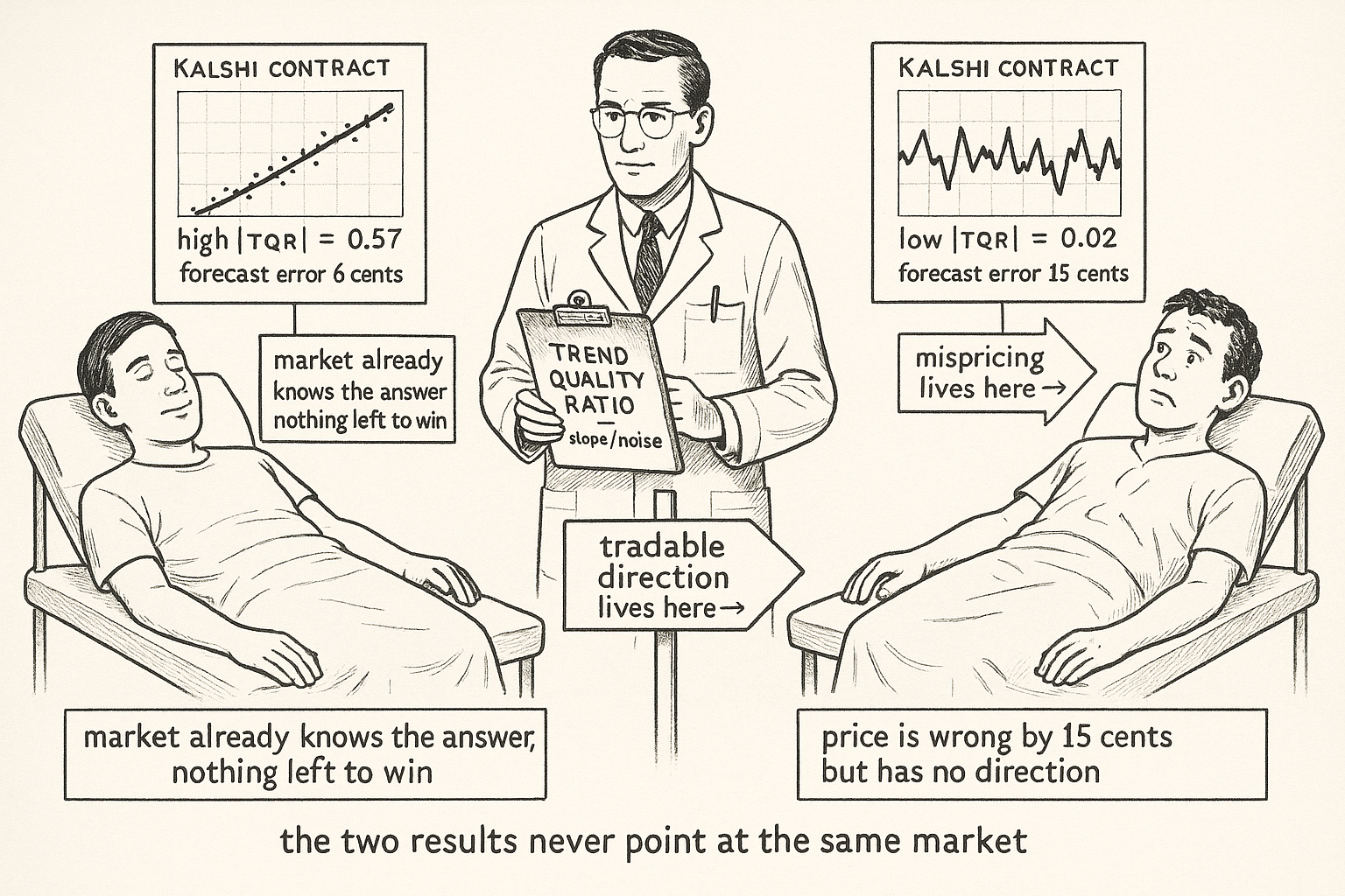
Second, and this is the part that decides whether TQR is tradable, low forecast error means the market price was already close to the truth. Deciles 4 and 5 show zero-change shares of 64.3% and 64.2%, the highest in the table, alongside the lowest errors. Those are contracts that have stopped trading because the answer is settled and the price is pinned near a boundary. Knowing that a price is accurate gives you nothing to bet on. You need the price to be wrong and to know which way. Low trend quality flags the contracts with the largest errors, so that is where the mispricing lives, and by construction those are the contracts with no discernible direction. The error result and the directional result point at disjoint sets of markets.
Midquotes erase the direction and keep the error
Greene rebuilds everything from the midpoint of the best bid and ask, which cures stale last trades and raises the usable sample from 18,987 to 21,464 contracts and the non-zero-trend set from 4,061 to 5,077. The two versions of TQR correlate at about 0.77, so this is the same statistic measured on a cleaner price.
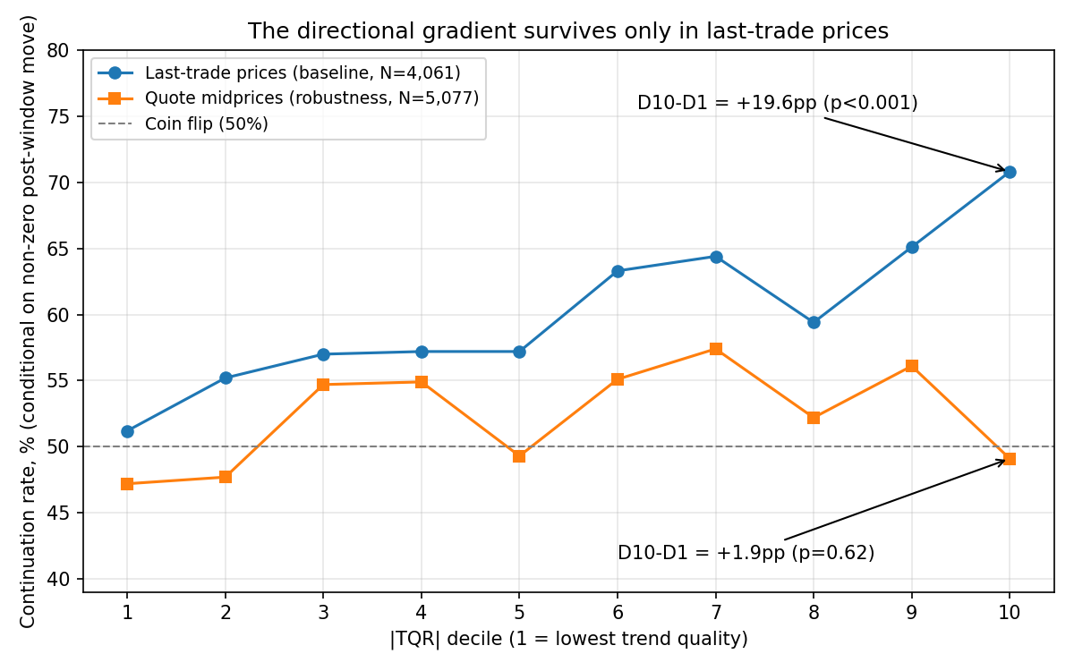
The directional gradient disappears. Top minus bottom falls to 1.9 points with a bootstrap p-value of 0.62, the tie-adjusted version falls to 1.4 points at p equal to 0.63, and the top decile itself prints 49.1%, under a coin flip. The out-of-sample classification result is worse than null: trend quality alone reaches an AUC of 0.448 on midquotes, against 0.583 on last trades. A ranker below 0.5 is ranking backwards. Meanwhile the price-level and spread controls, with no trend quality at all, reach an AUC of 0.617.
The error result survives the switch and gets larger, from 25.52 cents in the bottom decile to 5.51 in the top, a 78.4% cut. Read the rest of that column before crediting it to trend quality. In the midquote regression of absolute error on trend quality plus controls, mean spread carries a coefficient of 0.571 and the specification reaches an R-squared of 0.576, while adding trend quality contributes 0.005. Out of sample the controls deliver an R-squared of 0.311 and adding trend quality drops it to 0.291. Spread is doing the work. Wide-spread contracts are unresolved contracts trading in the middle of the range, and those carry large settlement errors for reasons that have nothing to do with how straight their last 18 minutes looked.
The baseline sample tells a quieter version of the same story. The decile sort gives 8.68 cents, but the conditional regression of absolute error on trend quality with controls gives a coefficient of minus 6.177 with a standard error of 3.259, so t equals minus 1.90. Multiply that coefficient by the 0.550 spread in mean |TQR| between the bottom and top deciles and you get minus 3.40 cents, which is 39% of the sorted gap and not significant at 5%. The continuation regression holds up better: 0.166 times 0.550 gives 9.1 points against the sorted 11.1.
The break-even the paper never runs
Take the top decile at face value and price the trade. Buy in the trend's direction at 12 minutes remaining, hold to close, exit at the prevailing price.
$$ \mathbb{E}[\pi] \;=\; \bigl(2\,\text{Cont}^{0.5} - 1\bigr)\,d \;-\; k \qquad\Longrightarrow\qquad d^{*} \;=\; \frac{k}{2\,\text{Cont}^{0.5} - 1} $$
Expected profit per contract in cents is the directional edge multiplied by d, the average absolute size of the post-window move in cents, minus k, the round-trip cost in cents from spread and fees. This assumes the winning and losing moves average the same size, which is generous near a boundary. The break-even move size d-star is the cost divided by the edge.
The top decile's edge is 2 times 0.619 minus 1, which is 0.238. At a 1-cent round trip you need the average post-window move to exceed 4.2 cents to break even, and at 2 cents you need 8.4 cents. Put a plausible 2-cent move through it and the gross take is 0.48 cents per contract, which a 1-cent round trip erases twice over. In the bottom decile the edge is 0.018 and the gross take on the same 2-cent move is 0.036 cents.
Whether d clears 4.2 cents cannot be answered from this paper, because the signed post-window change is defined and never tabulated, spread is carried as a control and never reported as a level, and no cost assumption appears anywhere in the text. Those three omissions are the gap between a state variable and a strategy.
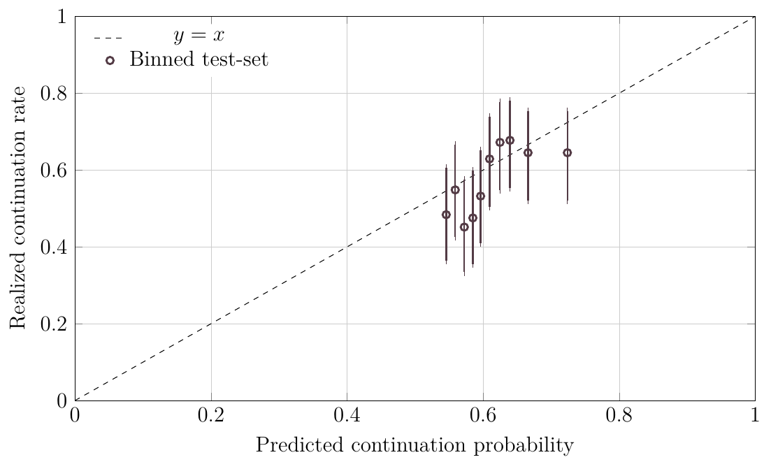
Greene's own reliability check says the same thing in a picture. Predicted continuation probabilities compress into the band from 0.54 to 0.72, the two highest-predicted bins both realize about 64.5% and so fall below their predictions, and every bin's 95% Wilson interval spans roughly 12 points. Nothing in that plot separates the contracts you would size up from the ones you would skip. Greene labels it a noisy check rather than a validation, which is the right call.
What TQR is actually for
Trend quality near settlement earns a place in a Kalshi dashboard as a convergence gauge. High absolute TQR on last trades says the market has picked a side and is walking to it, so there is little left to win and the post-window continuation you would be betting on is mostly the pin. Low absolute TQR says the price is still wrong by 12 to 15 cents on average and nobody knows which way, which is where mispricing sits and where a directional trend signal has nothing to say. Used as a filter for standing down, it costs nothing and it is cheap to compute from a bid, an ask and a timestamp.
Used as alpha it fails on the paper's own evidence. Out-of-sample R-squared is negative for both continuous targets in the baseline, from minus 0.003 to minus 0.019 on the tie-adjusted score and minus 0.017 to minus 0.064 on absolute error, which says a constant beats the model on held-out contracts. The AUC of 0.583 is the single number that survives, and it evaporates to 0.448 the moment you measure price from quotes rather than from the last trade someone happened to print. The direction result depends on stale transaction prices. Glosten and Milgrom explained why quotes and trades carry different information 40 years ago, and the sensible conclusion here is that a trend fitted to sporadic last trades in a thin near-expiry contract is partly measuring the arrival pattern of trades. Moskowitz, Ooi and Pedersen built time-series momentum across decades of futures data with cost models attached. An 18-minute regression on a contract that will not exist in 12 minutes is not in that category, and Greene says so in the discussion: TQR "should not be viewed as a universal alpha." That sentence is the finding.
KEY POINTS
- The Trend Quality Ratio is the pre-close trend slope divided by its residual RMSE on the window from 30 to 12 minutes before a Kalshi contract closes. The paper's two divisions by mean price cancel exactly, so the price-level normalization described in section 4.1 does nothing.
- TQR carries units of one over minutes, not the "dimensionless" score section 4.1 claims. The same path scores 0.4167 per minute and 0.00694 per second, so every decile threshold is tied to the 18-minute window and the minute clock. Treat this as a source error, not something to silently redefine.
- TQR equals the slope t-statistic divided by the square root of the regressor sum of squares. Same TQR of 0.4167 gives t equal to 9.41 on 19 prints and 4.59 on the 5-print minimum, so the sort ranks effect size and ignores how much data backs it.
- The headline direction result is a top-minus-bottom continuation gap of 19.6 points (70.8% against 51.2%). It conditions on the post-window move being non-zero, which you cannot filter on at entry, and Table 1 and Table 2 reconcile through the identity 2 times Cont-0.5 minus 1 equals (1 minus tie share) times (2c minus 1).
- The 8.68-cent forecast-error improvement (a 58.9% cut) points the wrong way for a trader. Low error means the price at 12 minutes was already right, and the lowest-error deciles are the pinned ones with 64% zero-change shares. Mispricing sits in the low-TQR contracts, which by construction have no direction.
- Rebuild from quote midprices and the direction dies: top minus bottom falls to 1.9 points at p equal to 0.62, the top decile prints 49.1%, and the trend-quality-only AUC falls to 0.448 while price and spread controls alone reach 0.617. Spread carries the midquote error result, with an R-squared of 0.576 and trend quality adding 0.005.
- Out-of-sample R-squared is negative on both continuous targets in the baseline, so a constant beats the model on held-out contracts. Break-even needs the average post-window move to clear 4.2 cents at a 1-cent round trip, and the paper never reports the move size, the spread level or any cost assumption.
- Sample caveats the paper discloses or implies: one BTC series supplies 89% of raw snapshots, only 1,094 of 4,061 non-zero-trend contracts resolved, per-decile resolved counts are never printed, and the midrange error result rests on about 23 resolved markets per decile.