8.9 Regime-Switching That Works, Factors That Don't (MS-GARCH)

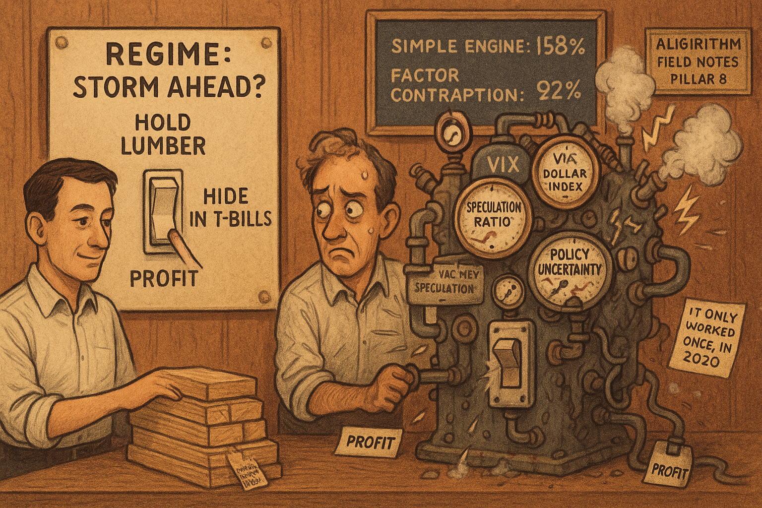
Regime-switching gets sold as the model that tells you when to leave. Turn it on, it flags the storm, you step aside before the drawdown. De la Torre-Torres, Álvarez-García, and del Río-Rama ran the honest version of that pitch on one commodity and reported every number, the ugly ones included. They traded random-length lumber futures weekly from 2004 to 2023 with a single rule: if a two-regime Markov-switching model says next week is high-volatility, sit in 3-month Treasury bills; otherwise hold lumber. The headline is a 158% cumulative return against 7% for buy-and-hold. The two results that actually teach you something sit underneath it.

The first: the entire edge depends on which variance model you bolt onto the regime switch, not on the regime switch itself. Swap the variance engine and the same rule goes from losing 53% to making 158%. The second: the authors then loaded the model with market and behavioral factors, expecting a lift, and the good versions got worse. The old article "Volatility-Regime Filter for Any Strategy" made the general case for gating any strategy by its volatility regime. This paper is that idea run through a real estimation engine on a real instrument, and it shows where the idea earns its keep and where the fancy version quietly breaks.

The rule is one inequality

The trader holds lumber or holds cash, nothing in between. Each week the model estimates the probability of being in the low-volatility regime (call it s=1) and the high-volatility regime (s=2), then projects that probability forward one week and checks a threshold. If the forecasted probability of the high-vol regime next week, written xi for s=2 at t+1, is 50% or lower, take a full long position in the 1-month lumber future. If it is above 50%, move 100% into the T-bill fund. The forecast itself is a matrix multiply on the current regime probabilities.

$$ \begin{bmatrix} \xi_{s=1,t+n} \\ \xi_{s=2,t+n} \end{bmatrix} = P^{n} \begin{bmatrix} \xi_{s=1,t} \\ \xi_{s=2,t} \end{bmatrix}, \qquad P = \begin{bmatrix} \pi_{11} & \pi_{12} \\ \pi_{21} & \pi_{22} \end{bmatrix} $$

Read it plainly. The vector on the right is where the model thinks you are right now: the smoothed probabilities of each regime at time t. P is the transition matrix, where each entry is the probability of moving from one regime to another. Raising P to the power n and applying it walks those probabilities n weeks ahead. For the trade you only need n equal to one, the one-week-ahead forecast.

Work a number. Say the model puts you at 80% low-vol and 20% high-vol today, so the current vector is 0.80 and 0.20. Suppose the transition matrix says low-vol stays low with probability 0.90 and flips to high with 0.10, while high-vol reverts to low with 0.30 and stays high with 0.70. The one-week high-vol forecast is 0.10 times 0.80 plus 0.70 times 0.20, which is 0.08 plus 0.14, or 0.22. That is 22%, below the 50% line, so you hold lumber into next week. The threshold is the whole discretion in the system. Everything hard happens upstream, in how the model decides those probabilities.

That matters because the benchmark is close to flat. Buy-and-hold lumber returned 7.13% over the full 1022-week sample, about 0.34% a year. Lumber went almost nowhere across two decades while whipping violently around that flat line. A rule that sidesteps the worst weeks has room to add a lot without predicting direction at all.

The variance model is the whole game

Here is where the paper stops being a lumber study and becomes a lesson about regime models. The authors did not test one model. They crossed three probability distributions for the likelihood (Gaussian, Student's t, and the fat-tailed generalized error distribution) with four ways of modeling the regime's volatility: a time-fixed variance, a plain ARCH, a symmetric GARCH, and an asymmetric EGARCH. Same rule, same data, twelve engines. The spread in results is enormous.

The time-fixed variance models, the ones that assume each regime has a constant volatility, were the worst. The Gaussian version lost 52.9% and the GED version lost 20.1%. The moment the variance is allowed to move within a regime, the picture flips. The symmetric GARCH models made 86% to 151%, and the asymmetric EGARCH with a GED likelihood topped the table at 158.3%. The mechanism is a time-varying variance recursion running inside each regime.

$$ \hat{\sigma}^2_t = \omega + \alpha\,\varepsilon^2_{t-1} + \beta\,\hat{\sigma}^2_{t-1} $$

The forecast variance today, sigma-squared-t, is a baseline omega, plus a reaction to yesterday's squared shock (alpha times epsilon-squared), plus a memory of yesterday's variance (beta times the prior sigma-squared). Alpha controls how sharply volatility jumps after a surprise; beta controls how long the elevated volatility lingers.

Work it. Set omega to 0.00002, alpha to 0.10, and beta to 0.85. Suppose last week delivered a 3% shock, so epsilon-squared is 0.0009, and the prior variance was 0.0004, a 2% weekly volatility. This week's variance is 0.00002 plus 0.10 times 0.0009 plus 0.85 times 0.0004, which is 0.00002 plus 0.00009 plus 0.00034, or 0.00045. Take the square root and volatility has climbed from 2.00% to 2.12%, and the 0.85 memory term keeps it elevated for weeks. The EGARCH variant goes one step further: it models the logarithm of variance and lets a negative shock raise volatility more than a positive shock of the same size. That asymmetry, the well-documented fact that lumber and most risk assets get more turbulent on the way down, is why the EGARCH caught the onset of high-vol regimes earlier and produced cleaner sell signals. A constant-variance regime model cannot see a storm building inside the calm regime; a GARCH one can.

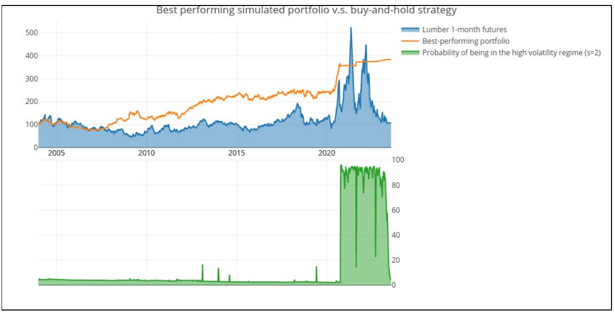
The lower panel is the tell. For most of the sample the forecasted high-vol probability sits near the floor, so the algorithm stays long. It spikes hard through the 2021-2022 lumber blow-off and collapse, and that is exactly when the model parks in T-bills while a buy-and-hold trader rides the price from roughly 500 back down to 100. The algorithm never forecasts price. It forecasts turbulence and refuses to hold through it.

Adding factors made the winners worse

The obvious next move is to feed the model more information. Instead of estimating regimes off lumber returns alone, estimate a mean equation first, packed with market and behavioral factors, and run the regime model on what is left over. The authors did exactly this, with the commodity-index return, Working's speculation ratio (volume over open interest), the VIX, and the dollar index as market factors, plus three sentiment trackers: economic policy uncertainty, a stock-market volatility news tracker, and an infectious-disease news tracker.

$$ \hat{r}_t = \alpha + \beta_1 \text{comm}_t + \beta_2 \text{WHR}_t + \beta_3 \text{VIX}_t + \beta_4 \text{DXY}_t + (\text{sentiment}) + \varepsilon_t, \qquad \varepsilon_t = r_t - \hat{r}_t $$

The first part fits a predicted return, r-hat-t, from the factors. The second part is the piece that matters: the Markov-switching GARCH model is estimated on the residual, epsilon-t, which is the actual return minus the factor prediction, not on the return itself. This is a structural constraint, not a choice. A GARCH process cannot be estimated jointly with a moving mean because of path dependence, so the factors are forced into the mean equation and the regime model only ever sees the leftovers.

Work it. Suppose lumber returns 1.2% one week and the factor model predicts 0.5%. The residual fed to the regime model is 0.7%. Change the factor set and every residual in the history changes, which means the regimes the model detects change too. That is the trap. Richer factors do not sharpen the volatility signal; they redraw the entire residual series the volatility model learns from.

The result was blunt. Factors helped the models that did not work and hurt the ones that did. The broken time-fixed MS models jumped (the Student's t version posted 282%, the highest number in the paper), but the authors trace that spike almost entirely to the single 2020 COVID episode, not to any repeatable skill. The GARCH and EGARCH engines that carried the no-factor results went backward: GARCH with a GED likelihood fell from 151% to 92.6%, and the EGARCH-GED winner dropped from 158.3% to 123.5%.

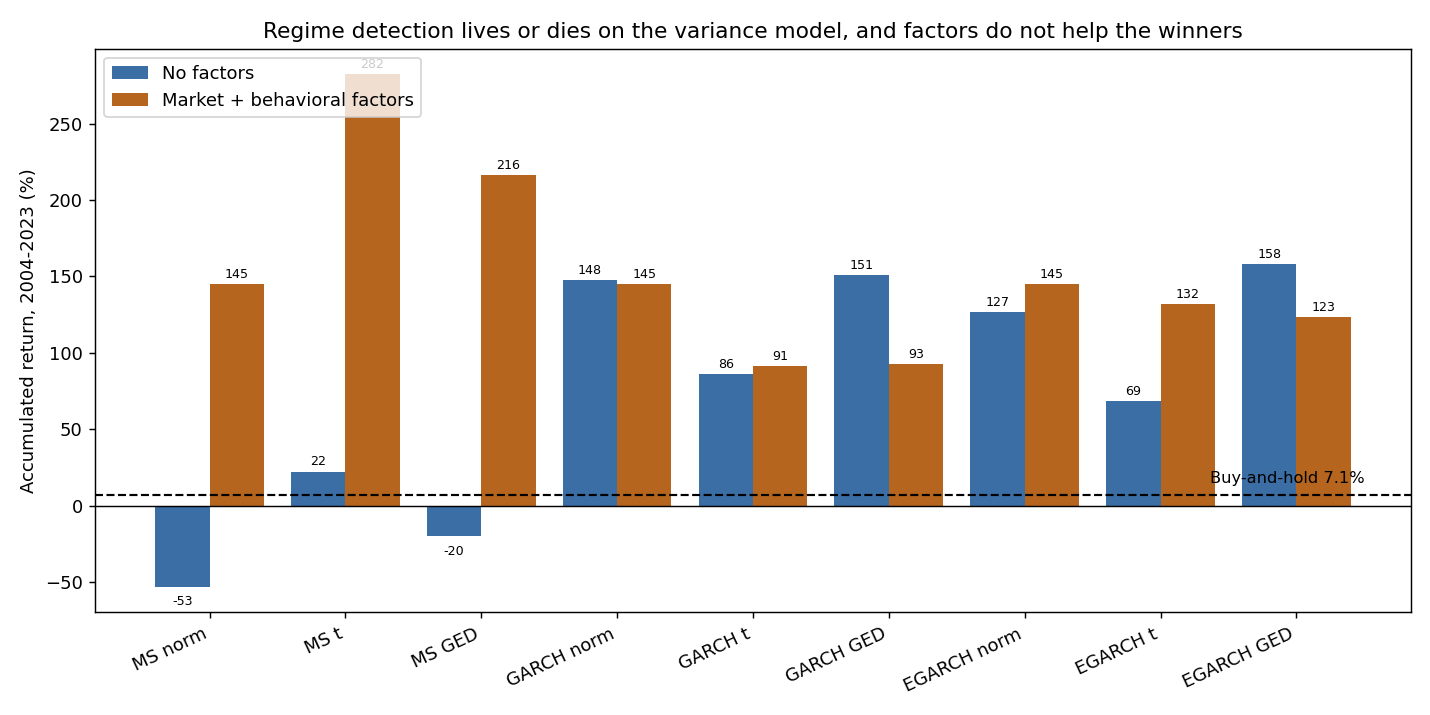
This is a clean instance of the old article "Loose Pants Fit Everyone: Why General Trading Ideas Survive Longer." The lean model, lumber returns and nothing else, generalized. The tailored model, seven factors and three sentiment indexes stitched into the mean, fit its residuals to a narrower set of past conditions and lost ground where it counted. The authors set out to prove that factors help (their Hypothesis 2) and reported, against their own thesis, that they do not.

The alpha that mostly wasn't

The 158% headline needs a second look before anyone builds on it. The paper measures skill with Jensen's alpha against the broad commodity futures market, which strips out the return you got just for holding a commodity when commodities happened to rise.

$$ \alpha = r_t - \beta\, r_{m,t} $$

Alpha is the portfolio return, r-t, minus its market exposure beta times the commodity-market return, r-m-t. If alpha is positive by a meaningful amount, the algorithm added something the market did not hand it for free. Work it: a 0.12% weekly portfolio return, a beta of 0.9, and a 0.10% commodity-market week give alpha of 0.12% minus 0.09%, or 0.03% per week, roughly 1.6% a year.

That 0.03% is close to what the winning model actually earned in alpha terms, and it is thin. Only three of the nine no-factor portfolios posted any positive alpha at all; the rest matched or lagged the broad commodity market. The winner's Sharpe ratio was 0.059, barely off zero. The rule beats buy-and-hold, but buy-and-hold was a flat 0.34% a year, so clearing it is a low bar. Measured against the thing that pays you nothing for skill, the broad commodity index, most of these portfolios added almost nothing. The regime switch is real and it dodges crashes; the risk-adjusted excess return on top of just owning commodities is small.

What the backtest quietly leaves out

Two omissions decide whether any of this survives contact with a broker. The authors state plainly that no trading fees were included. A rule that flips 100% in and 100% out on a weekly signal churns hard, and on an illiquid contract the round-trip cost is not a rounding error. Strip the fees out and the thin 1.6%-a-year alpha has to cover a spread it never paid in the simulation.

The bigger problem is the instrument. CME wound down the random-length lumber contract in 2023, right where the sample ends, and replaced it with a smaller, differently specified lumber future. The exact series tested here stopped trading. On top of that, this is one commodity, one sample, with the "best fitting" variant chosen each week by an in-sample information criterion, which is a form of selection the out-of-sample story has to carry. The transferable lesson is not "trade lumber this way." It is the structural finding: gate an asset by a regime model, put the effort into an asymmetric time-varying variance, and resist the urge to feed the model factors that only redraw its residuals. The regime switch worked because of the variance engine. The factors failed because they never touched it.

KEY POINTS

• The strategy is one inequality: if the forecasted probability of next week's high-volatility regime is 50% or lower, hold lumber; otherwise hold 3-month T-bills. The forecast is the current regime probabilities pushed one step through the transition matrix.
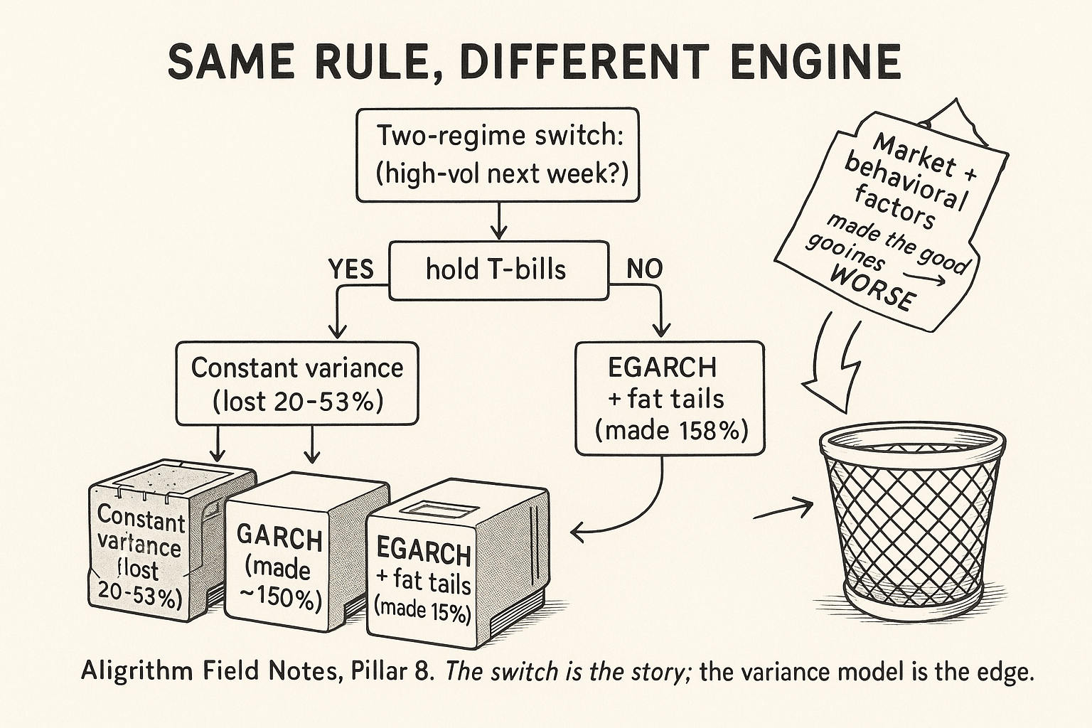
• The edge lives in the variance model, not the regime switch. Constant-variance regime models lost 20% to 53%; symmetric GARCH made 86% to 151%; the asymmetric EGARCH with a fat-tailed GED likelihood topped out at 158.3% against 7.1% for buy-and-hold.
• Asymmetry is why EGARCH won. Modeling log-variance and letting negative shocks raise volatility more than positive ones caught the onset of turbulent regimes earlier and produced cleaner exits, visible in the 2021-2022 lumber crash.
• Adding market and behavioral factors backfired on the models that worked. Factors enter only through the mean equation, so the regime model is fit on residuals; richer factors redraw those residuals and dragged GARCH-GED from 151% to 92.6% and EGARCH-GED from 158% to 123.5%.
• The 282% factor "winner" was a broken time-fixed model rescued by a single 2020 COVID episode, not repeatable skill.
• The alpha is thin. Against the broad commodity index most portfolios added almost nothing; the winner's Sharpe was 0.059 and its alpha near 0.03% a week. Beating a flat 0.34%-a-year buy-and-hold is a low bar.
• The backtest charged no trading fees on a weekly full-flip rule, and the tested random-length lumber contract was discontinued in 2023. Treat the transferable result as a method, not a lumber trade.

References

• A New Approach to the Economic Analysis of Nonstationary Time Series and the Business Cycle (Hamilton, 1989)
• A New Approach to Markov-Switching GARCH Models (Haas, Mittnik, and Paolella, 2004)
• Generalized Autoregressive Conditional Heteroskedasticity (Bollerslev, 1986)
• Conditional Heteroskedasticity in Asset Returns: A New Approach (Nelson, 1991)
• Forecasting Risk with Markov-Switching GARCH Models: A Large-Scale Performance Study (Ardia, Bluteau, Boudt, and Catania, 2018)
• The Trading Profitability of Forecasts of the Gilt-Equity Yield Ratio (Brooks and Persand, 2001)
• Error Bounds for Convolutional Codes and an Asymptotically Optimum Decoding Algorithm (Viterbi, 1967)
• An EM/MCMC Markov-Switching GARCH Behavioral Algorithm for Random-Length Lumber Futures Trading (De la Torre-Torres, Álvarez-García, and del Río-Rama, 2024)

A note on AI. The ideas, research, analysis, and conclusions in this article are my own. I use AI tools to help with editing and wordsmithing, because English is not my first language, and I am not shy about that. AI-generated ideas and AI-assisted writing are not the same thing: the first is empty slop from a generic prompt, the second is a tool for communicating years of real research more clearly. Judge the work by its substance, not by whether software helped polish the prose.